
Time-domain instability mechanism for artificial boundary condition of semi-infinite medium described by discrete rational approximation
 0
0Abstract
The use of discrete rational approximation functions to represent foundation dynamic impedance plays a crucial role in the time-domain analysis of soil-structure interaction regarding artificial boundary. In modeling, the rational approximation functions need to be transformed into time-domain recursive models for incorporation into time-history analysis. However, this method also suffers from uncertainties in parameter identification and instability in time-domain analysis when the time-domain recursive models of soil are coupled with upper structure. The stability issue in artificial boundary coupled time-domain computation has not been effectively addressed. This paper establishes the closed-loop transfer function of the coupled system and analyzes the causes of instability in the coupled system based on gain margin analysis. Different numerical simulations demonstrate that the major cause of artificial boundary system instability is the description errors of discrete rational approximation functions beyond the fitting frequency range.
Keywords
INTRODUCTION
Soil-structure interaction (SSI) has an obvious effect on the seismic response of many structures, such as high-rise buildings[1], nuclear power plants[2], ocean structures[3], and long-span bridges[4]. Currently, when dealing with SSI problems, it is a common practice to divide the soil into a near-field finite domain and a far-field infinite domain. In addressing the far-field infinite domain, an artificial convex-shaped boundary is introduced to simulate the actual boundary conditions of the far-field soil. And frequency response functions are often used to represent the influence of the semi-infinite far-field soil on the near-field finite domain. Various time-domain methods are used to convert the frequency response functions into time-domain mechanical models, which are coupled with the superstructure for time-domain analysis. Currently, commonly used time-domain methods include continued fraction expansion[5-7], operator split methods[8], rational approximation function[9-13], etc. Among them, according to the computation time, the rational approximation method, compared to other current time-domain methods, is characterized by its simplicity and high applicability. It is not restricted by variations in the research subject, and it can also describe the frequency response function effectively, even at lower orders. In addition, this method demonstrates a combination of high precision and straightforward computational procedures. As a result, it has gained widespread attention and extensive research by scholars.
Rational approximation functions can be divided into discrete-time rational approximation functions[14] and continuous-time rational approximation functions[15]. The stability and accuracy of rational approximation functions and their corresponding time-domain mechanical models[16-20] are consistent within the fitting frequency range. Therefore, the accurate and stable identification results of discrete-time rational approximation functions are the key to ensuring the effectiveness of time-domain calculations of the recursive models. Wolf and Motosaka[21] used curve fitting techniques based on least squares methods to convert frequency-domain discrete rational approximation functions into time-domain recursive equations and pointed out that the stability condition of the function is that the poles are within the unit circle in the complex plane. Paronesso and Wolf[22] started from the unit impulse response matrix of the semi-infinite medium and derived the time-domain recursive equation by using balanced approximation methods to calculate the interaction forces of discrete-time rational approximation functions. When fitting discrete rational approximation functions, Wang et al. eliminated unstable solutions by imposing penalty terms on the objective function and retained stable solutions[23,24]; in addition, they converted them into rational approximation functions with the same stability by using bilinear transformation. However, stable discrete-time mechanical models cannot guarantee the stability of the overall system after coupling with the structure. Laudon et al. proposed a method to evaluate the stability of the coupled system, which is combined with a numerical integration method and a recursive parameter model[25]. He used the method to represent the dynamic characteristic of the base system and validated that stable time-domain calculations of the Safak model[19] can still lead to instability after being coupled with structures. Gash et al. pointed out that even if the filter and the employed time integration method are stable, we cannot guarantee that their combination is also stable[26]. He derived the stability expression for the filter-integrator combination process by combining discrete-time rational approximation functions with numerical integration algorithms. After comparing the stability of rational approximation models with the stability of coupled systems, Lesgidis et al. found that the constraints only for the rational approximation model could not guarantee that the globally coupled dynamic system is absolutely stable[27]. Saitoh effectively implemented the interaction of system motion and guaranteed the stability of the coupled system by introducing lumped parameter models to represent impedance functions[28,29]. Zhao et al. combined the standard dynamic finite element method for the complex near field and the high-order accurate artificial boundary conditions for the simple far field to obtain symmetric second-order coupled dynamical equations with diagonal mass matrix and non-diagonal damping matrix[30], gave the multi-degree-of-freedom (MDOF) continuous-time lumped parameter model, resolved the instability issue after coupling by introducing a Rayleigh damping proportional to the stiffness matrix, and put it into the finite element model of the finite domain.
When scholars deal with the instability issue in calculating artificial boundary problems using discrete-time rational approximation functions, most studies only considered the stability of the rational approximation functions themselves. Some scholars have pointed out that time-domain models transformed from stable rational approximation functions can still become unstable when coupled with structures and integrated into the time domain. For this issue, they only provided judgment methods for the stability of coupled systems. This paper targets the instability problem occurring in discrete-time rational approximation functions and numerical computation of coupled structures. The closed-loop transfer function of the coupled system is established to analyze the instability mechanism of artificial boundary systems based on the concept of gain margin.
SYSTEM STABILITY OF ARTIFICIAL BOUNDARY COUPLED WITH STRUCTURE
Stability of discrete-time rational approximation functions
In SSI analysis, the artificial boundary conditions are used to replace the far-field infinite domain and simulate its wave radiation effect. Furthermore, using frequency response functions to describe the interaction relationship of infinite domain medium-structure systems is a common method for solving artificial boundary problems. The frequency response functions of the infinite domain include the dynamic stiffness coefficient S(ω) of the far-field infinite domain and its reciprocal flexible coefficient F(ω). The interaction relationship between infinite medium and structure can be expressed as:
In the equation, the vector f(ω) is the generalized force; u(ω) is the generalized displacement; the dynamic stiffness function S(ω) can be expressed as the following frequency-dependent function:
In the equation, ω is the frequency of external load; S0 is the static stiffness;
The artificial boundary system is a linear time-invariant discrete (LTID) system but not a differential system, thus being difficult to solve in the time domain. In order to obtain a differential description of the artificial boundary system, using the bilinear transformation method in Ref.[14] to convert the discrete-time filter in Ref.[19] into the following discrete-time rational approximation:
where S0 is the static stiffness; bk (k = 0, …, N) and ak (k = 1, …, M) are the undetermined coefficients of the numerator and denominator of the function, respectively; z = eiωΔt is the Z-transform frequency domain symbol; i is the imaginary unit; ω is the frequency of external load; Δt is the discrete-time step.
Since the time-domain mechanical models and the frequency domain rational approximation functions have the same stability and accuracy, high-precision rational approximation functions that meet the stability requirements need to be obtained in the parameter identification phase. According to linear control theory, the stability condition of Equation (1) is that the modulus of all poles of the denominator is less than 1. Let
After obtaining a stable rational approximation function, in order to introduce it into the artificial boundary system for time-domain analysis, it needs to be converted into an equivalent time-domain recursive filter through inverse Fourier transform[15]. The discrete-time recursive filter is a simple finite difference equation; it converts a given time sequence (i.e., input) into another time sequence (i.e., output). The discrete-time recursive filter is defined by the following equation:
where u(t) represents the input of the filter as displacement; after filtering, the output is fl(t), M, N are the orders of the filter, bi and ai represent the coefficients of the filter, and t is time.
Instability phenomenon of the coupled system
Under the premise of ensuring the stability of the soil model, it was found that instability phenomenon would occur after the coupling between the soil model and the structure. A simple single-degree-of-freedom (SDOF) structure shown in Figure 1 is used here to illustrate the instability phenomenon of the coupled system. The horizontal motion frequency response function of the circular foundation is shown in Figure 2; it is identified using discrete-time rational functions, with parameters taken from Ref.[15]. Some foundation parameters are: foundation radius r = 30 m, soil shear modulus G = 0.3 × 10⁹ Pa, soil Poisson’s ratio v = 1/3, and density ρ = 1,600 kg/m3. The discrete-time rational approximation is 5th order. The structural mass is

Figure 1. Horizontal motion of structure-circular foundation.
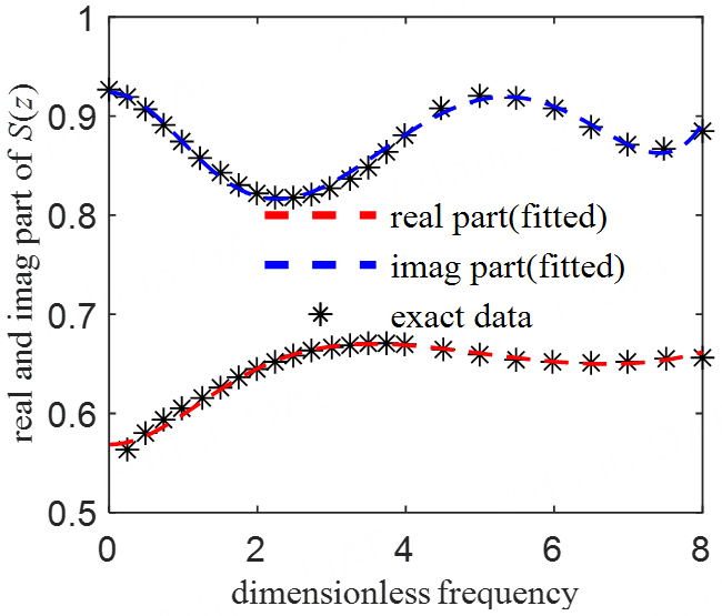
Figure 2. Structure-circular foundation parameter identification results.

Figure 3. Structure-circular foundation time history analysis results.
Identification of accuracy and efficiency of circular foundation
| Order | 3 | 5 | 7 | 9 | 11 |
| Error (%) | 16.82 | 12.29 | 7.49 | 6.74 | 6.62 |
| Time of calculation (s) | 4.46 | 4.19 | 5.79 | 7.12 | 8.66 |
As shown in Table 2, by constraining the coefficient within the stable interval, the identified poles all have magnitudes less than 1. The data satisfies the stability theorem. However, it can be seen from Figure 3 that the time history of the coupled artificial boundary system is diverging, resulting in instability.
Identification of parameters and poles of denominator in rational approximation function
| Parameter identification results | Magnitude of poles | |
| b0 | 11.3337 | |
| b1 | -15.8584 | |
| b2 | 4.6624 | |
| b3 | -3.7880 | |
| b4 | 6.4099 | |
| b5 | -2.2653 | |
| a1 | 0.8847 | 0.6857 |
| a2 | -0.9304 | 0.6816 |
| a3 | -0.8300 | 0.8595 |
| a4 | 0.2164 | 0.7109 |
| a5 | 0.1947 | 0.6816 |
COUPLED SYSTEM INSTABILITY ANALYSIS METHOD
Coupled system transfer function
After obtaining the time-domain mechanical model shown in Equation (5), We can establish the artificial boundary system shown in Figure 4. The dynamic equation of the system is shown in Equation (6):

Figure 4. Artificial boundary system computational model.
In the equation, M, C, and K represent the mass, damping, and stiffness matrices, respectively; the subscripts s and b represent the structure and foundation, respectively;
As mentioned in Section "Instability phenomenon of the coupled system", a stable time-domain recursive model cannot guarantee the stability of the coupled system. In order to facilitate the analysis of the instability mechanism of the coupled system, a transfer function between the structural displacement and the seismic displacement is derived based on Z-transform for a SDOF rational approximation system. The structural displacement mainly consists of two parts, namely, the sum of the displacement generated by the foundation under seismic action and the displacement generated by the time-domain recursive force of the infinite domain medium interacting on the foundation. Letting the transfer function between the foundation displacement u and the time-domain recursive force F of the medium act on the foundation be G1, the transfer function between the structural displacement Xne and the seismic displacement xg be G2, and the transfer function between the structural displacement Xf and the external force be G3, then the displacement generated by the structure is:
Moving the second term on the right side of Equation (7) to the left side of the equation and rearranging, the transfer function between the structural displacement and the seismic displacement is obtained as:
The system flowchart is shown in Figure 5:
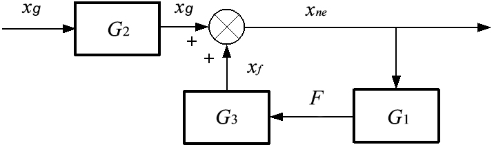
Figure 5. Closed-loop block diagram of the coupled system.
In order to achieve an exact solution for function (8), we solve for G1, G2, and G3 separately. The transfer function G1 between the time-domain recursive force and the foundation displacement is the discrete-time rational approximate function obtained using the genetic-sequential quadratic programming algorithm.
The transfer function G2 between the structural relative displacement and the seismic displacement can be calculated by structural dynamic equation:
Performing the Z-transform on the obtained dynamic equation allows us to derive the following formula:
Where m, c, and k represent the mass, damping, and stiffness of the structure, respectively. The transfer function G3 between the structural relative displacement and the external force can be obtained by the same method as for G2:
When using the dynamic equilibrium equation to solve the relative displacement of the foundation, since the displacement for each step has not been determined when calculating the time-domain recursive force for that step, the displacement from the previous step needs to be used to calculate the recursive force for the current step. Therefore, G1 will produce a one-step time lag error. To eliminate the error caused by the one-step time lag in the frequency domain, when constructing the overall transfer function H, G1 will take the following form:
Equation (8) can be expressed as:
A 3 × 3 pile group foundation shown in Figure 6 is used as an example; we investigate a SDOF structure to validate the accuracy of the constructed transfer function. The pile diameter d = 1 m, pile spacing s = 5 m, pile length L = 6 m, soil Poisson’s ratio ν = 0.35, and soil damping ratio β = 0.05. The SDOF structure has mass m = 7.3 × 10⁷ kg, stiffness k = 4.6 × 10¹⁰ N/m, and damping ratio of 0.05. Under seismic action, calculate the transfer function and numerical integration results. Use the genetic-sequential quadratic programming algorithm to fit the dynamic stiffness curve of pile groups. It is then converted into the time-domain recursive force between the semi-infinite medium and the foundation using the time-domain recursion algorithm[17]. The fitting results are shown in Figure 7 and Table 3.
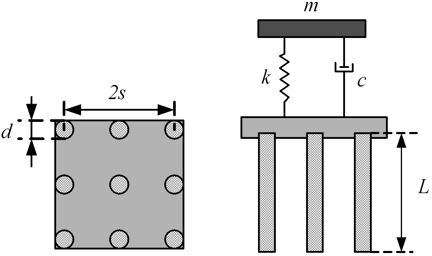
Figure 6. 3 × 3 pile group foundation model.
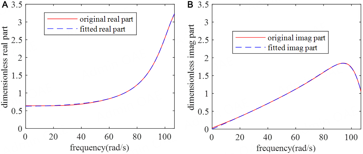
Figure 7. 5th order rational function approximation identification results of pile group foundation. (A) Real part of impedance; (B) imaginary part of impedance.
Identification impedance parameters of 3 × 3 pile group foundation
| Numerator coefficients | Data | Denominator coefficients | Data |
| b0 | 3.9129 | a1 | 1.0209 |
| b1 | -4.8201 | a2 | 0.9188 |
| b2 | 9.3310 | a3 | 0.7100 |
| b3 | -7.5729 | a4 | 0.6541 |
| b4 | 3.7882 | a5 | 0.3912 |
| b5 | -1.6806 |
Using the ground motion of the El Centro earthquake as input, the displacement of the artificial boundary system structure is calculated by the Newmark-β method. The output of the coupled system transfer function system constructed is calculated in MATLAB. The calculation results are compared, as shown in Figure 8. The peak error is 2.9673 × 10⁻¹³. Therefore, the correctness of the established frequency domain transfer function can be verified.

Figure 8. Displacement time histories of foundation calculated by transfer function algorithm and time-domain recursive algorithm under seismic excitation.
Gain margin analysis
According to the control theory principle, the stability of a closed-loop system is determined by the open-loop characteristic equation[31,32]. The closed-loop characteristic equation (13) determining the stability of the control-based coupled system is:
In order to comprehensively judge the instability mechanism of a SDOF system, gain margin[33] analysis of the magnitude-frequency and phase-frequency characteristics can be adopted for the SDOF system. As shown in Figure 9, the gain margin is defined as the reciprocal of the magnitude at the crossover frequency where the phase angle is -180°. The critical stability condition of the system is when the gain margin equals 1 at the crossover frequency. When the gain margin is less than 1, the system is stable, and when the gain margin is greater than 1, the system is unstable, with the degree of instability increasing as the gain margin increases.

Figure 9. Principle of gain margin. (A) Phase; (B) magnitude.
Based on this, the crossover frequency ωGM and gain margin GM of the system can be calculated according to the following equation:
INSTABILITY MECHANISM OF COUPLED SYSTEM
Sampling theorem
According to the sampling theorem[34], the sampling frequency of a discrete-time system must be greater than twice the highest frequency of the signal.
The equation has been shown in Equation (17). In this case, the discrete points obtained through sampling can restore the sampled signal relatively accurately. If the sampling frequency is less than or equal to twice the highest frequency of the signal, it will lead to aliasing in the sampled signal. Aliasing should be avoided when sampling the system.
Taking the sine wave signal shown in Figure 10 as an example, this illustrates the necessity of Equation (17). If four sample points are taken within half a cycle, and the sampling rate is eight times the signal frequency, the signal characteristic can be restored basically. If the sampling rate is reduced to the critical point,

Figure 10. Sampling results with different sampling frequencies. (A) Fs = 8F; (B) Fs = 2F; (C) Fs < 2F.
Distortion of fitting
When using discrete-time rational approximation functions to fit the frequency response function, due to the limitation of fitting accuracy, usually only functions within a limited frequency band (0~ωf) are fitted, as shown in Figure 11. Therefore, the obtained rational approximation function can accurately reproduce the base impedance within the fitting frequency band, while the out-of-band components (ω > ωf) still exist in numerical calculation. And the magnitude of the fitted function will generate a large peak at the Nyquist frequency[35] ωN, leading to notable discrepancies between the magnitude of the fitted function and the original function. This phenomenon will cause distortion of the recovered signal.

Figure 11. Contrast of magnitude of rational approximation function and the original function.
Numerical example
Numerical example 1. analysis of a cylinder in water
Taking a cylinder with a diameter R = 8 m and depth h = 80 m in water shown in Figure 12 as an example to analyze the relationship between the sampling frequency band length and system stability. The sound speed in water is taken as c = 1,438 m/s, and the water density ρ = 1,000 kg/m3. The El Centro earthquake is the external load excitation.

Figure 12. Cylinder in infinite domain water.
In order to verify the influence of different fitting frequency bands on the calculation accuracy of the system, we use the rational approximation function to fit the dynamic stiffness of the cylindrical in water. The original magnitude and phase of the coupled system are then compared with the magnitude and phase of the fitted function. The maximum values of the fitting frequency band are taken as 10, 15, and 20 Hz. And it is used respectively for parameter fitting, frequency domain, and time-domain calculations. The calculation results are shown in Figure 13 and Table 4.
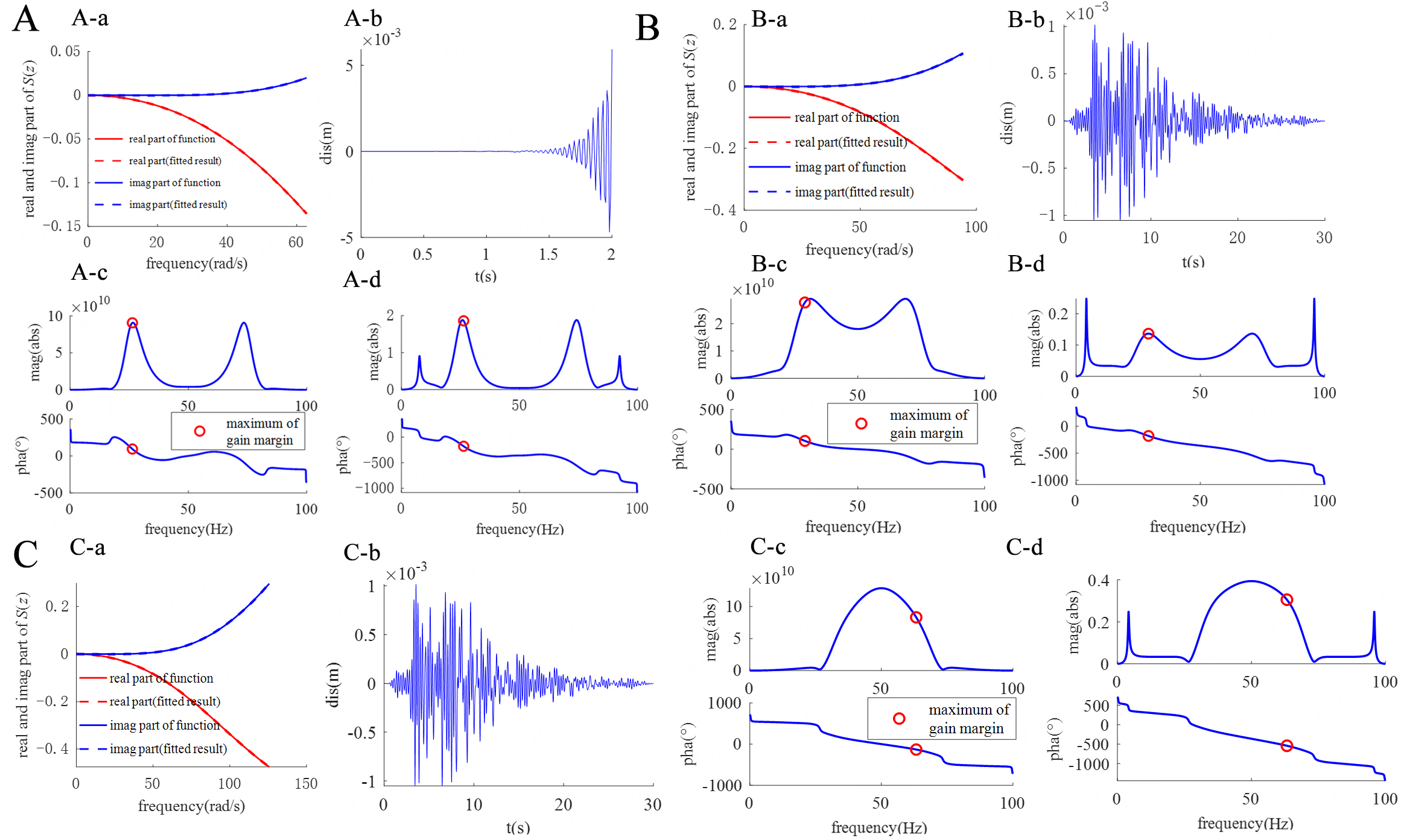
Figure 13. Analysis results of frequency domain and time domain under different fitting frequency bands of infinite domain water. (A) 0~10 Hz: (A-a) Parameter fitting result of cylinder in water; (A-b) Time history result of cylinder in water; (A-c) Infinite water domain frequency domain characteristic; (A-d) Water-structure interaction system frequency domain characteristic; (B) 0~15 Hz: (B-a) Parameter fitting result of cylinder in water; (B-b) Time history result of cylinder in water; (B-c) Infinite water domain frequency domain characteristic; (B-d) Water-structure interaction system frequency domain characteristic; (C) 0~20 Hz: (C-a) Parameter fitting result of cylinder in water; (C-b) Time history result of cylinder in water; (C-c) Infinite fluid domain frequency domain characteristic; (C-d) Fluid-structure interaction system frequency domain characteristic.
Frequency domain analysis results of systems with different fitting frequency bands of infinite domain water
| Maximum value of the fitting frequency band (Hz) | Frequency at maximum margin ωf (Hz) | Maximum magnitude of rational function | Original frequency response function | Gain margin |
| 10 | 26.33 | 9.0436 × 10¹⁰ | 5.6435 × 10⁹ | 1.8613 |
| 15 | 29.14 | 2.9032 × 10¹⁰ | 6.4825 × 10⁹ | 0.1364 |
| 20 | 63.24 | 1.2857 × 10¹¹ | 1.4843 × 10¹⁰ | 0.3055 |
It can be seen from Figure 13 that when the maximum fitting frequency band is 10, 15, and 20 Hz, the parameter identification results have high accuracy. The rational approximation function magnitude-frequency dynamic characteristic shows a large error outside the fitting frequency band. According to Table 4, at the frequency where the gain margin is maximum, the magnitude of the rational approximation function is greater than the original frequency response function. When the maximum fitting frequency is 10 Hz, the system becomes unstable.
In order to analyze the fitting error between the obtained rational function and the original frequency response function, the dynamic characteristic of the rational approximation function identification results and the original frequency response function in the frequency range of 0~100 Hz are compared when the maximum fitting frequency band is 10~20 Hz. The comparison results are shown in Figure 14.
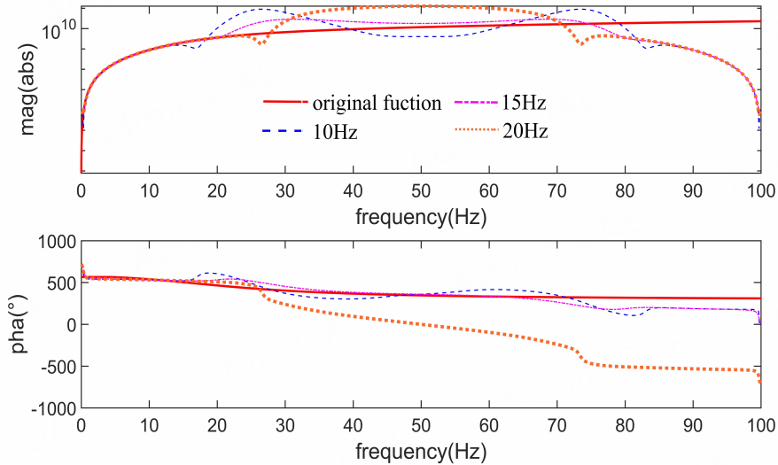
Figure 14. Comparison of dynamic characteristic of frequency response function and rational approximation function of infinite domain water.
It can be seen from Figure 14 that within the fitting frequency band, the dynamic characteristic of the obtained rational approximation function fits well with the original frequency response function, while outside the fitting frequency band, large errors in the magnitude values are observed. For the unstable condition of 0~10 Hz, the magnitude at the unstable frequency is 9.0436 × 10¹⁰, while the magnitude of the original frequency response function at this frequency is 5.6435 × 10⁹. The magnitude differs by 16 times, indicating severe distortion in the frequency domain characteristic. As a result, the gain margin of the system is much greater than 1, and the system becomes unstable. Thus, the reason for instability is that the rational approximation function exhibits significant distortion compared to the original frequency response function outside the fitting frequency range.
Numerical example 2. analysis of a circular foundation
In order to further analyze the influence of fitting errors on system stability, gain margin is used to analyze the system stability shown in Figure 1. We perform gain margin analysis on the SDOF artificial boundary system within the frequency range of 0~100 Hz, as shown in Table 5. The maximum gain margin value for this system is 2.15, as marked in the figure, and the corresponding unstable frequency is 56.96 Hz.
Frequency domain analysis of SDOF coupled system
| Unstable frequency of the system (Hz) | Base impedance magnitude | Structure magnitude | Coupled system magnitude |
| 56.96 | 5.88 × 10¹² | 3.65 × 10⁻¹³ | 2.15 |
It can be seen from Figure 15A that the base impedance obtained through parameter identification has a peak magnitude near the Nyquist frequency (50 Hz). At the Nyquist frequency, the phase of the discrete rational approximation function is 0, while the phase angle of the dynamic characteristic of the base structure shown in Figure 15B at this frequency is about -180°. Due to the one-step delay error, the phase angle of the rational approximation function changes. However, the phase at this frequency point is near 0, thus causing the crossover frequency at which the system becomes unstable to be near the Nyquist frequency. From Table 5, at the unstable frequency 56.96 Hz, the magnitude of the rational approximation function is 5.88 × 10¹², and the magnitude of the frequency domain characteristic of the structure is

Figure 15. Frequency domain analysis of horizontal motion coupled system of circular foundation. (A) SDOF coupled system frequency domain characteristic of base impedance; (B) SDOF coupled system frequency domain characteristic of structure; (C) SDOF coupled system gain margin analysis of coupled system; (D) Comparison of frequency domain characteristics between rational function and original data.
Due to the need of structural dynamic analysis, when fitting the rational approximation function, the frequency range of the fitted frequency response function is limited to a narrow frequency band. In the above example, the frequency response function within 0~18.37 Hz was fitted quite accurately. However, the rational function obtained from parameter identification produces a large magnitude error at the Nyquist frequency outside the fitting frequency band, as shown in Figure 15D. According to modern control theory, if the maximum sampling frequency of the system is less than the Nyquist frequency of the system, large errors caused by signal aliasing can be avoided. And the original signal can be restored more accurately. Therefore, the peak appearing at the Nyquist frequency outside the fitting frequency band of the discrete rational approximation function greatly affects the stability of the system.
PARAMETER ANALYSIS TO THE COUPLED SYSTEM STABILITY
Effect of soil shear modulus on coupled system stability
It can be seen from the above content that the magnitude characteristic of the base impedance function has a great influence on system stability. The magnitude of the impedance function is related to the shear modulus of the soil. In order to analyze the influence of shear modulus on system stability, the horizontal motion frequency response function of the circular foundation in Section "Instability phenomenon of the coupled system" is used as the dynamic characteristic of the foundation. The foundation radius r = 30 m, shear modulus G takes

Figure 16. Dynamic characteristic of soils with different soil shear moduli.

Figure 17. Dynamic characteristic of coupled system with different soil shear moduli.
Coefficients of rational approximate functions for horizontal motion of circular foundations
| j | 0 | 1 | 2 | 3 | 4 | 5 |
| aj | 1 | 0.7064 | -1.0032 | -0.7087 | 0.2515 | 0.1777 |
| bj | 13.1450 | -19.9613 | 6.0497 | -2.0115 | 5.3438 | -2.1744 |
Frequency domain analysis of systems with different soil shear moduli
| Shear modulus (N/m) | 1.5 × 10⁸ | 2.0 × 10⁸ | 2.5 × 10⁸ |
| Maximum of gain margin (Hz) | 64.23 | 58.05 | 56.91 |
| Magnitude at the maximum of gain margin | 7.6708 × 10¹¹ | 3.1157 × 10¹² | 5.6447 × 10¹² |
| Gain margin | 0.3295 | 1.1577 | 2.0612 |
According to Figures 16 and 17, Table 7, when the shear modulus of the soil takes different values, the instability frequency of the system is around 60 Hz, indicating that the shear modulus of the soil has little influence on the instability frequency of the system. As the shear modulus increases, the magnitude of the dynamic characteristic of the soil increases significantly. This is because the larger the shear modulus, the greater the static stiffness of the rational approximation function, corresponding to the larger magnitude of the dynamic characteristic of the soil. The gain margin of the system also increases accordingly.
Effect of structural parameters on coupled system stability
In order to analyze the effect of structural parameters on system stability, the fitting results of the horizontal motion frequency response function of the circular foundation in Section "Instability phenomenon of the coupled system" are adopted. Different artificial boundary systems are established by changing the structural parameters to carry out stability analysis.
Effect of structural frequency on system stability
In order to study the effect of structural frequencies on the stability of the coupled system, the structural stiffness k = 4.6 × 10¹⁰ N/m, and the damping ratio = 0.05. By altering the mass of the upper structure, the frequency of the structure can be modified to fall within the range of 2~8 Hz. By studying the changes in gain margin at different structural frequencies, we can assess its impact on the instability of coupled systems. The dynamic characteristics of the structure under different frequencies are shown in Figure 18. The frequency domain analysis under different working conditions is shown in Figure 19 and Table 8.
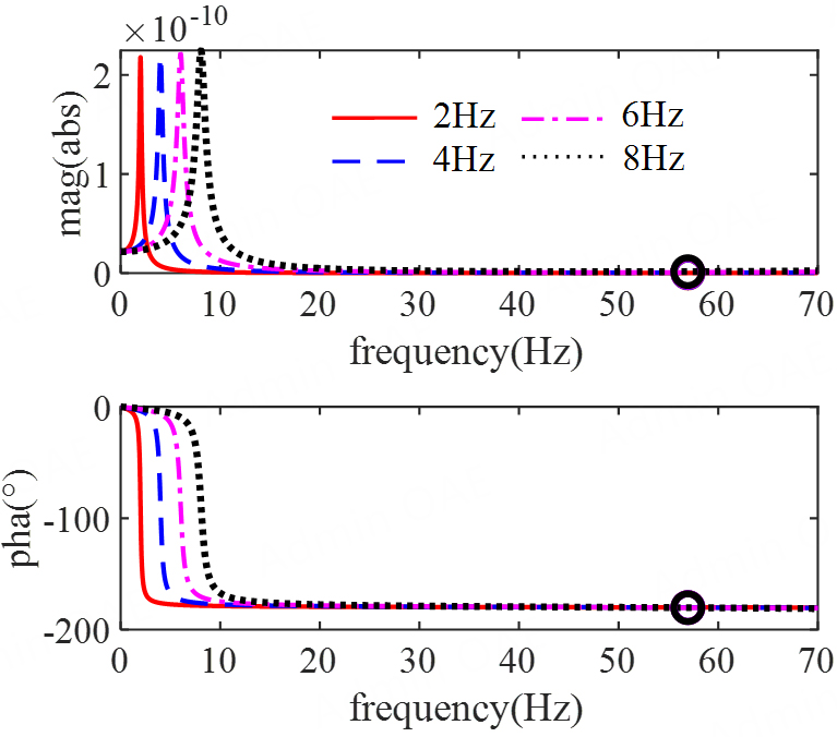
Figure 18. Dynamic characteristic of structure with different structural frequencies.

Figure 19. Dynamic characteristic of coupled system with different frequencies.
Frequency domain analysis of systems with different structural frequencies
| Structural frequency (Hz) | 2 | 4 | 6 | 8 |
| Maximum of gain margin (Hz) | 59.59 | 59.57 | 59.55 | 59.52 |
| Magnitude at the maximum of gain margin | 9.45 × 10⁻¹⁴ | 3.83 × 10⁻¹³ | 8.81 × 10⁻¹³ | 1.62 × 10⁻¹² |
| Gain margin | 0.1876 | 0.7642 | 1.7673 | 3.2690 |
From Figure 18, it can be seen that the phase change of the structure at the instability frequency is very small. The instability frequencies of the system under different working conditions are all around 59.5 Hz, indicating that the frequency of the structure basically does not affect the instability frequency. From Table 8, it can be seen that as the structural frequency increases, the magnitude in the frequency domain dynamic characteristic of the structure increases, and the gain margin of the artificial boundary system also increases correspondingly. When the structural frequency is within 4 Hz, the system is stable, and when it is 6 Hz or above, the system becomes unstable. This shows that high-frequency structures are more likely to cause artificial boundary system instability.
Effect of structural damping ratio on system stability
The structural stiffness k = 4.6 × 10¹⁰ N/m, and the structural mass m = 5.754 × 10⁷ kg. To study the influence of structural damping ratio on the stability of the coupled system, the structural damping ratio is designed to be 0.01~0.07. Using the same method as studying structural frequencies, investigate the impact of structural damping ratios on the stability of coupled systems. The dynamic characteristics of the structure at different frequencies are shown in Figure 20. The frequency domain analysis under different working conditions is shown in Figure 21 and Table 9.

Figure 20. Dynamic characteristic of structure with different structural damping ratios.
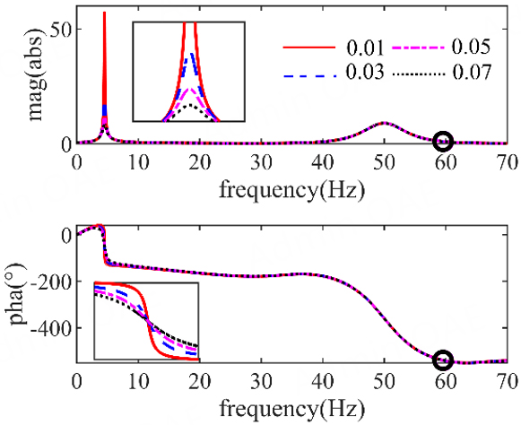
Figure 21. Dynamic characteristic of coupled system with different structural damping ratios.
Frequency domain analysis of system with different structural damping ratios
| structural damping ratio | 0.01 | 0.03 | 0.05 | 0.07 |
| Maximum of gain margin (Hz) | 59.60 | 59.58 | 59.56 | 59.54 |
| Magnitude at the maximum of gain margin | 4.87 × 10⁻¹³ | 4.8701 × 10⁻¹³ | 4.8681 × 10⁻¹³ | 4.8661 × 10⁻¹³ |
| Gain margin | 0.9643 | 0.9693 | 0.9743 | 0.9793 |
Based on Figures 20 and 21, Table 9, when the structure takes different damping ratios, the magnitude and phase of the structure change very small at the instability frequency. The instability frequencies of the system under different working conditions are around 59.5 Hz, and the gain margin is around 0.97, indicating that the damping ratio of the structure has little effect on the stability of the artificial boundary system.
Effect of discrete-time step on coupled system stability
In order to analyze the effect of s discrete-time step Δt on system stability, the fitting results of the horizontal motion frequency response function of the circular foundation in Section "Instability phenomenon of the coupled system" are adopted. Taking time steps of Δt = 0.005, 0.01, and 0.02 s, using the rational approximation function to fit the original frequency response function. The El Centro earthquake is the external excitation, and we perform time history and gain margin analysis.
From Figure 22, it can be observed that the fitting results for all three discrete-time steps meet the requirement, so there is no significant error due to fitting inaccuracies. Analyzing the displacement time history from Figure 22, it is evident that as the discrete-time step increases, the coupled system transitions from stability to instability, and the instability point occurs earlier. Through Table 10, it can be seen that with the increase in the discrete-time step, the frequency at which the maximum gain margin occurs shifts to lower values. In addition, the gain margin of the system increases from 0.5288 to 4.9717. This phenomenon indicates that higher discrete-time steps are more likely to lead to instability in the coupled system.
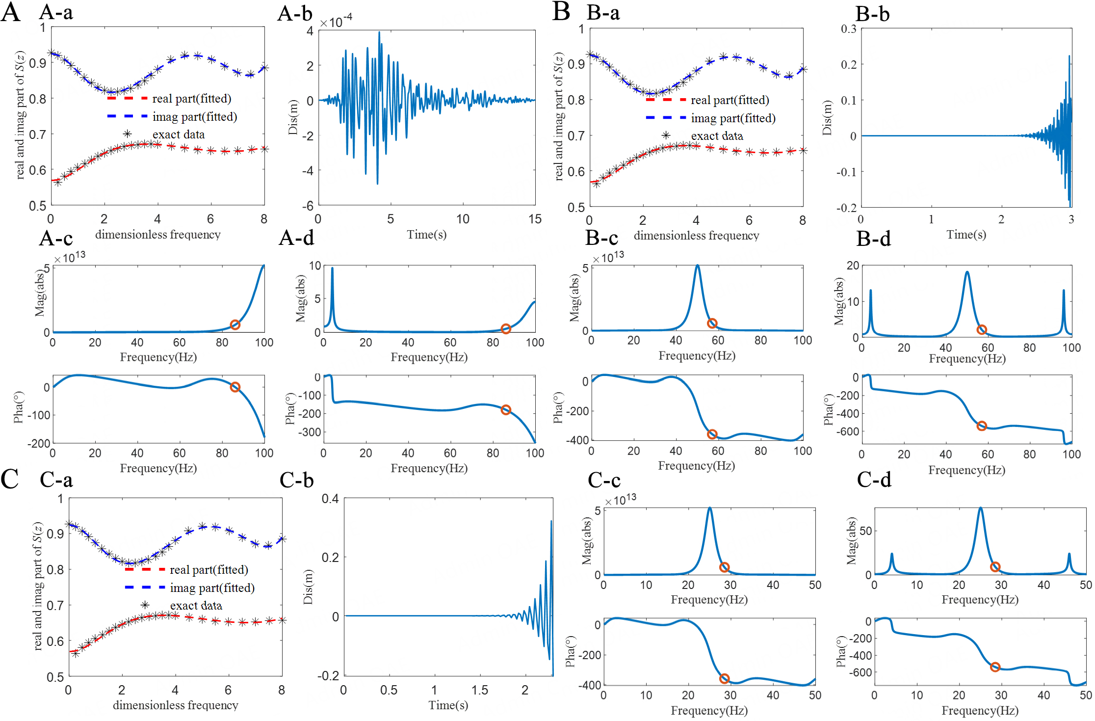
Figure 22. Analysis results of frequency domain and time domain under different discrete-time steps of structure-circular foundation. (A) Δt = 0.005 s: (A-a) Parameter fitting result of circular foundation; (A-b) Time history result of circular foundation; (A-c) Infinite soil domain frequency domain characteristic; (A-d) Soil-structure interaction system frequency domain characteristic; (B) Δt = 0.01 s: (B-a) Parameter fitting result of circular foundation; (B-b) Time history result of circular foundation; (B-c) Infinite soil domain frequency domain characteristic; (B-d) Soil-structure interaction system frequency domain characteristic; (C) Δt = 0.02 s: (C-a) Parameter fitting result of circular foundation; (C-b) Time history result of circular foundation; (C-c) Infinite soil domain frequency domain characteristic; (C-d) Soil-structure interaction system frequency domain characteristic.
Frequency domain analysis of system with different discrete-time steps
| Discrete-time step (s) | 0.005 | 0.01 | 0.02 |
| Maximum of gain margin (Hz) | 86.06 | 56.96 | 28.47 |
| Magnitude at the maximum of gain margin | 5.86 × 10¹² | 5.881 × 10¹² | 5.922 × 10¹² |
| Gain margin | 0.5288 | 2.1489 | 9.1123 |
CONCLUSION
In order to understand the instability issue of the coupled system of discrete rational approximation artificial boundary and superstructure, this paper proposes a method to explain the instability mechanism of the artificial boundary coupled system based on the concept of gain margin. Through different numerical examples, the effect of soil characteristics, structural characteristics, and discrete-time steps on system stability is analyzed. The main conclusions are as follows:
(1) The closed-loop transfer function of the SDOF artificial boundary system is established. Based on the concept of gain margin and the closed-loop transfer function, an instability mechanism analysis method of the coupled system of discrete rational approximation artificial boundary and upper structure is proposed in frequency domain.
(2) Theoretical analysis and numerical simulation demonstrated that the instability frequency of the coupled system is out of the fitting frequency range for discrete rational approximation function and near the Nyquist frequency. Therefore, it can be shown that the main reason causing the instability of the coupled system is that the magnitude of the discrete rational approximation function appears to be a large peak outside the fitting frequency range, which seriously distorts the dynamic characteristic of the converted time-domain model in the high frequency range. Thus, the description of discrete rational approximation functions obviously causes errors for the artificial boundary system beyond the fitting frequency range.
(3) The effect of shear moduli of soil, frequency and damping ratios of different structures, and discrete-time steps on the stability of the coupled system is analyzed. Numerical simulation results show that the increase of soil shear modulus leads to the increase of static stiffness of soil, and the magnitude of discrete rational approximation function increases accordingly. The stability of the coupled system decreases with the increase of structural frequency, while the structural damping ratio has little effect on the system stability. As the discrete-time step increases, the gain margin of the coupled system also increases significantly; the coupled system becomes more prone to instability, which is detrimental to the stability of the artificial boundary system.
(4) Meanwhile, this paper has the following limitations: The rational approximation function can only address linear problems within the frequency domain and is unable to account for the nonlinearity of the soil. In addition, this passage only focuses on the instability issues of the medium under single deformation such as horizontal and sway, without considering its behavior under coupled deformations. We will address this issue in future work.
DECLARATIONS
Acknowledgments
The authors gratefully acknowledge the support of the China Scholarship Council.
Authors’ contributions
Project administration, methodology: Tang Z
Writing, validation: Fu B
Data curation, research design: Li X
Availability of data and materials
Not applicable.
Financial support and sponsorship
None.
Conflicts of interest
All authors declared that there are no conflicts of interest.
Ethical approval and consent to participate
Not applicable.
Consent for publication
Not applicable.
Copyright
© The Author(s) 2024.
REFERENCES
1. Zhang X, Far H. Effects of dynamic soil-structure interaction on seismic behaviour of high-rise buildings. Bull Earthq Eng 2022;20:3443-67.
2. Han SR, Nam MJ, Seo CG, Lee SH. Soil-structure interaction analysis for base-isolated nuclear power plants using an iterative approach. J Earthq Eng Soc Korea 2015;19:21-8.
3. Zuo H, Bi K, Hao H. Dynamic analyses of operating offshore wind turbines including soil-structure interaction. Eng Struct 2018;157:42-62.
4. Cao J. Dynamic characteristic analysis considering of pile-soil-superstructure interaction based on long-span cable-stayed bridge. Appl Mech Mater 2012;178-81:2497-500.
5. Wu WH, Lee WH. Nested lumped-parameter models for foundation vibrations. Earthq Eng Struct Dyn 2004;33:1051-8.
6. Wang J, Zhou D, Liu W, Wang S. Nested lumped-parameter model for foundation with strongly frequency-dependent impedance. J Earthq Eng 2016;20:975-91.
7. Sun Y, Zhou D, Amabili M, Wang J, Han H. Liquid sloshing in a rigid cylindrical tank equipped with a rigid annular baffle and on soil foundation. Int J Str Stab Dyn 2020;20:2050030.
8. Liu T, Zhao C. Finite element modeling of wave propagation problems in multilayered soils resting on a rigid base. Comput Geotech 2010;37:248-57.
9. Ruge P, Trinks C, Witte S. Time-domain analysis of unbounded media using mixed-variable formulations. Earthq Eng Struct Dyn 2001;30:899-925.
10. Cazzani A, Ruge P. Numerical aspects of coupling strongly frequency-dependent soil-foundation models with structural finite elements in the time-domain. Soil Dyn Earthq Eng 2012;37:56-72.
11. Cazzani A, Ruge P. Rotor platforms on pile-groups running through resonance: a comparison between unbounded soil and soil-layers resting on a rigid bedrock. Soil Dyn Earthq Eng 2013;50:151-61.
12. Cazzani A, Ruge P. Symmetric matrix-valued transmitting boundary formulation in the time-domain for soil-structure interaction problems. Soil Dyn Earthq Eng 2014;57:104-20.
13. Cazzani A, Ruge P. Stabilization by deflation for sparse dynamical systems without loss of sparsity. Mech Syst Signal Process 2016;70-1:664-81.
14. Zhao M, Du X. Stability and identification for rational approximation of foundation frequency response: discrete-time recursive evaluations. Eng Mech 2010;27:141-7. Available from: https://www.engineeringmechanics.cn/en/article/id/883 [Last accessed on 31 Jan 2024]
15. Du X, Zhao M. Stability and identification for rational approximation of foundation frequency response: continuous-time lumped-parameter models. Eng Mech 2009;26:76-084. Available from: https://www.engineeringmechanics.cn/en/article/id/815 [Last accessed on 31 Jan 2024]
16. Wolf JP, Somaini DR. Approximate dynamic model of embedded foundation in time domain. Earthq Eng Struct Dyn 1986;14:683-703.
17. Wolf JP. Consistent lumped-parameter models for unbounded soil: physical representation. Earthq Eng Struct Dyn 1991;20:11-32.
18. Wu WH, Lee WH. Systematic lumped-parameter models for foundations based on polynomial-fraction approximation. Earthq Eng Struct Dyn 2002;31:1383-412.
19. Şafak E. Time-domain representation of frequency-dependent foundation impedance functions. Soil Dyn Earthq Eng 2006;26:65-70.
20. Wang H, Liu W, Zhou D, Wang S, Du D. Lumped-parameter model of foundations based on complex Chebyshev polynomial fraction. Soil Dyn Earthq Eng 2013;50:192-203.
21. Wolf JP, Motosaka M. Recursive evaluation of interaction forces of unbounded soil in the time domain from dynamic-stiffness coefficients in the frequency domain. Earthq Eng Struct Dyn 1989;18:365-76.
22. Paronesso A, Wolf JP. Recursive evaluation of interaction forces and property matrices from unit-impulse response functions of unbounded medium based on balancing approximation. Earthq Eng Struct Dyn 1998;27:609-18. Available from: https://ui.adsabs.harvard.edu/abs/1998EESD...27..609P/abstract [Last accessed on 31 Jan 2024]
23. Wang P, Zhao M, Li H, Du X. An accurate and efficient time-domain model for simulating water-cylinder dynamic interaction during earthquakes. Eng Struct 2018;166:263-73.
24. Du X, Zhao M. Stability and identification for rational approximation of frequency response function of unbounded soil. Earthq Eng Struct Dyn 2010;39:165-86.
25. Laudon AD, Kwon OS, Ghaemmaghami AR. Stability of the time-domain analysis method including a frequency-dependent soil-foundation system. Earthq Eng Struct Dyn 2015;44:2737-54.
26. Gash R, Esmaeilzadeh Seylabi E, Taciroglu E. Implementation and stability analysis of discrete-time filters for approximating frequency-dependent impedance functions in the time domain. Soil Dyn Earthq Eng 2017;94:223-33.
27. Lesgidis N, Kwon OS, Sextos A. A time-domain seismic SSI analysis method for inelastic bridge structures through the use of a frequency-dependent lumped parameter model. Earthq Eng Struct Dyn 2015;44:2137-56.
28. Saitoh M. Simple model of frequency-dependent impedance functions in soil-structure interaction using frequency-independent elements. J Eng Mech 2007;133:1101-14.
29. Saitoh M. On the performance of lumped parameter models with gyro-mass elements for the impedance function of a pile-group supporting a single-degree-of-freedom system. Earthq Eng Struct Dyn 2012;41:623-41.
30. Zhao M, Li H, Du X, Wang P. Time-domain stability of artificial boundary condition coupled with finite element for dynamic and wave problems in unbounded media. Int J Comput Methods 2019;16:1850099.
31. Tao CS, Chang CH, Han KW. Gain margins and phase margins for multivariable control systems with adjustable parameters. Int J Control 1991;54:435-52.
32. Tang Z, Dietz M, Hong Y, Li Z. Performance extension of shaking table-based real-time dynamic hybrid testing through full state control via simulation. Struct Control Health Monit 2020;27:e2611.
33. Hong Y, Tang Z, Liu H, Li Z, Du X. Gain-margin based discrete-continuous method for the stability analysis of real-time hybrid simulation systems. Soil Dyn Earthq Eng 2021;148:106776.
34. Vaidyanathan PP. Generalizations of the sampling theorem: Seven decades after Nyquist. IEEE Trans Circuits Syst I 2001;48:1094-109.
Cite This Article
Export citation file: BibTeX | RIS
OAE Style
Tang Z, Fu B, Li X. Time-domain instability mechanism for artificial boundary condition of semi-infinite medium described by discrete rational approximation. Dis Prev Res 2024;3:2. http://dx.doi.org/10.20517/dpr.2023.38
AMA Style
Tang Z, Fu B, Li X. Time-domain instability mechanism for artificial boundary condition of semi-infinite medium described by discrete rational approximation. Disaster Prevention and Resilience. 2024; 3(1): 2. http://dx.doi.org/10.20517/dpr.2023.38
Chicago/Turabian Style
Tang, Zhenyun, Boxin Fu, Xin Li. 2024. "Time-domain instability mechanism for artificial boundary condition of semi-infinite medium described by discrete rational approximation" Disaster Prevention and Resilience. 3, no.1: 2. http://dx.doi.org/10.20517/dpr.2023.38
ACS Style
Tang, Z.; Fu B.; Li X. Time-domain instability mechanism for artificial boundary condition of semi-infinite medium described by discrete rational approximation. Dis. Prev. Res. 2024, 3, 2. http://dx.doi.org/10.20517/dpr.2023.38
About This Article
Copyright

Data & Comments
Data
0

 Cite This Article 5 clicks

 Like This Article 4
likes
Like This Article 4
likes


Comments
Comments must be written in English. Spam, offensive content, impersonation, and private information will not be permitted. If any comment is reported and identified as inappropriate content by OAE staff, the comment will be removed without notice. If you have any queries or need any help, please contact us at support@oaepublish.com.