
Stochastic stress response and dynamic reliability evaluation for transmission towers with semi-rigid behaviors
 0
0Abstract
As a kind of typical wind-sensitive structure, transmission towers have attracted fast-growing attention in the field of their wind-induced dynamic response. Nevertheless, their dynamic response considering effects of semi-rigid connected joints and semi-rigid-constrained stability behaviors has not been investigated. To this end, based on the experimental and numerical study, this paper proposes a fitting formula for the stability coefficient of steel tube members with semi-rigid behaviors in transmission towers to determine the dynamic stress response. Then, the stiffness, mass, and damping matrices of steel-tube transmission towers (STTTs) with semi-rigid behaviors are determined to construct their stochastic dynamic finite element model. Subsequently, the integral form of the generalized density evolution equation is solved via a family of Dirac's sequences to conduct the stochastic stress response analysis for STTTs considering effects of semi-rigid connected joints and semi-rigid-constrained stability behaviors, and their dynamic reliability is evaluated by further introducing the extreme-value distribution method. Finally, an engineering example of an existing STTT is given, and the results indicate that the semi-rigid connected joints and semi-rigid-constrained stability behaviors would significantly affect the stochastic stress response and dynamic reliability of STTTs. Accordingly, taking into account semi-rigid connected joints and semi-rigid-constrained stability behaviors may be more applicable for analysis and design of STTTs.
Keywords
INTRODUCTION
With the fast-growing demand for power supply in modern society, there is a huge need for building steel towers for transmitting electric power. Thus, it is quite crucial for transmission towers to reliably perform uninterrupted operation without any failure, among which steel-tube transmission towers (STTTs) have been widely constructed due to the same sectional performances in all directions and small windward areas. As a type of high-rise structure, the main load acting on transmission towers is a time-variant wind load owing to natural turbulence and gustiness in the wind. Therefore, it is essential to investigate the wind-induced dynamic response of transmission towers.
In the last two decades, some studies on the dynamic response of transmission towers under wind excitations have been comprehensively investigated. Savory et al. conducted a dynamic analysis of a latticed transmission tower under high-intensity wind loads[1]. Okamura et al. conducted a wind tunnel test to describe the wind characteristics in mountainous areas and carried out the response analysis of a transmission tower on the basis of the examinations[2]. Battista et al. studied the dynamic behavior of transmission line towers under wind loads and proposed a rational procedure for stability assessment in the design stage[3]. Yang and Hong carried out the nonlinear inelastic response analysis of a transmission tower-line system under downburst wind[4]. Moreover, Zhang and Xie studied the dynamic response of a transmission tower-line system, including the stress and displacement under strong wind loads[5]. Shen et al. and Li et al. studied the effect of conductor and insulator breakages on the dynamic response of transmission tower-line systems, respectively[6,7]. Additionally, some studies[8–14] focused on the determination of dynamic characteristics (e.g., modal parameters) of tower structures, and other research efforts[15,16] aimed to conduct the size and shape optimization and wind-induced vibration control for guyed structures. Furthermore, owing to the uncertainties associated with wind loads, materials, and dimensions, structural responses of transmission towers would exhibit random characteristics. Liu et al. proposed a dimension-reduced probabilistic approach to consider the stochastic wind fields for wind-induced dynamic response analysis of transmission towers, and the results indicated that the stochastic dynamic response of transmission towers induced by stochastic wind loads exhibited time-variant and random characteristics[17]; however, they did not consider the uncertainty of structures. The aforementioned studies mainly focus on the deterministic wind-induced dynamic response of transmission towers instead of their stochastic dynamic response. Therefore, it is necessary to comprehensively conduct the stochastic dynamic response analysis of transmission towers.
It is noted that latticed transmission towers have two specific features: (1) the joint is made using more than one bolt to form semi-rigid connections[18]; (2) the stability behavior of compression members in transmission towers would be influenced by the semi-rigid boundary constraint[19]. Accordingly, the semi-rigid connected joints and semi-rigid-constrained stability behaviors would affect the stochastic dynamic response (especially the stress of members) of transmission towers, which could further influence the dynamic reliability evaluation. Regretfully, to the best of the author's knowledge, there is a lack of relevant work on the structural stochastic response analysis and reliability evaluation of STTTs considering effects of semi-rigid connected joints and semi-rigid-constrained stability behaviors.
In response to this gap, this paper conducts the stochastic stress response analysis and dynamic reliability evaluation of STTTs, with a particular focus on considering the impact of semi-rigid connected joints and semi-rigid-constrained stability behaviors. The contributions of this paper are drawn below. (1) Based on the experimental and numerical study, a fitting formula for the stability coefficient of steel tube members with semi-rigid behaviors (STMs-SRB) in transmission towers is proposed to determine the dynamic stress response; (2) By solving the integral form of the generalized density evolution equation (GDEE)[20] via a family of Dirac's sequences and further introducing the extreme-value distribution approach[20], a method of stochastic stress response analysis and dynamic reliability evaluation is developed for STTTs considering the influence of semi-rigid connected joints and semi-rigid-constrained stability behaviors. The remaining content of this work is organized as follows. At first, a fitting formula for the stability coefficient of STMs-SRB is proposed to calculate their dynamic stress. Secondly, the stochastic stress analysis and reliability evaluation for STTTs considering effects of semi-rigid connected joints and semi-rigid-constrained stability behaviors is introduced. Then, an engineering example is given to investigate the effects of semi-rigid connected joints and semi-rigid-constrained stability behaviors on the stochastic stress response and dynamic reliability of transmission towers. Finally, Section 5 presents a summary of the key conclusions.
DYNAMIC STRESS RESPONSE OF STMS-SRB IN TRANSMISSION TOWERS CONSIDERING EFFECT OF STABILITY BEHAVIORS
Brief review of semi-rigid connected joints in STTTs
In STTTs, tube-gusset K-joints are specially designed to connect main chords and branch tubes, as illustrated in Figure 1. In detail, the K-joint consists of the main chord, branch tubes, C-type inserted plates, annular plates, gusset plates, and bolts for connecting gusset and C-type inserted plates. Therefore, this kind of K-joint is actually a semi-rigid connected joint, and its rotational stiffness
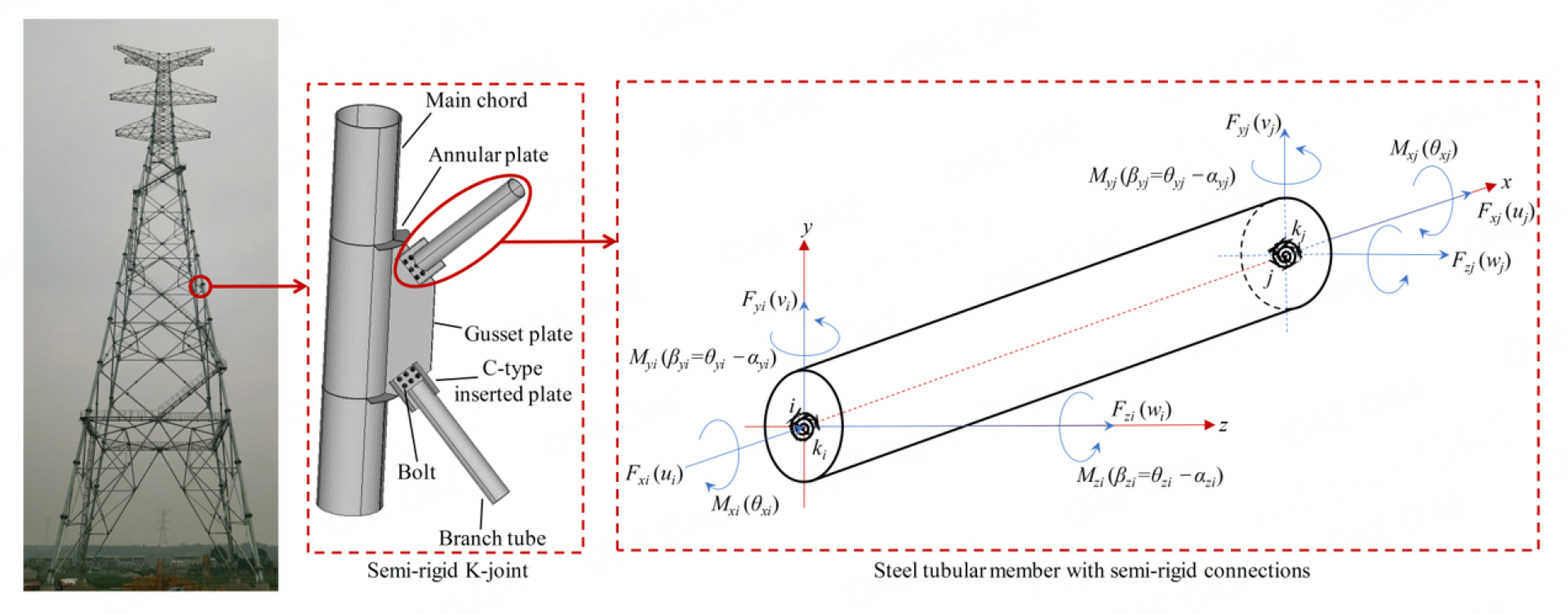
Figure 1. K-joint and steel tube member with semi-rigid behaviors.
Fitting formula for stability coefficient of STMs-SRB
Since the joint of STTTs is determined as a semi-rigid connection, the steel tube connected by this joint can be regarded as a member with semi-rigid behaviors. In our previous work[19], the experimental investigation and the numerical analysis have been conducted to study the stability behavior of STMs-SRB, and their comparison shows that the numerical analysis results fit well with the experimental results, as shown in Figure 2.

2. Comparison of experimental investigation and numerical analysis for stability behaviors of STMs-SRB.
In order to assess the bearing capacity of STMs-SRB by a fitting formula of the stability coefficient, the parametric numerical analysis is conducted in this paper by adopting the verified FE model of STMs-SRB, and the numerical analysis results could be further as a sample set to fit the stability coefficient of STMs-SRB. The varying parameters of the parametric numerical analysis include the rotational stiffness and the slenderness ratio, in which the rotational stiffness is taken as 50.99 kN
where
Combined with the least squares fitting method and the quadratic polynomial regression, the fitting formula for the stability coefficient
where
Fitting results of
| Rotational stiffness (kN | |||
| 50.99 | 11.2097 | -3.8505 | 1.3778 |
| 102.32 | 9.2400 | -3.0463 | 1.2905 |
| 201.34 | 7.1850 | -2.3429 | 1.2288 |
| 333.06 | 5.7896 | -1.9502 | 1.2063 |
The comparison of the stability coefficient between fitting and numerical results is shown in Figure 3A. It can be observed that the fitting results are in good agreement with the numerical results, and the maximum relative error is 2.8%. In addition, within the range of rotational stiffness, the stability coefficient can be obtained by the linear interpolation. The prediction of the stability coefficient by the proposed fitting formula is shown in Figure 3B, and the maximum relative error is 2.2%, indicating that the proposed fitting formula has satisfactory accuracy in predicting the stability coefficient of STMs-SRB.
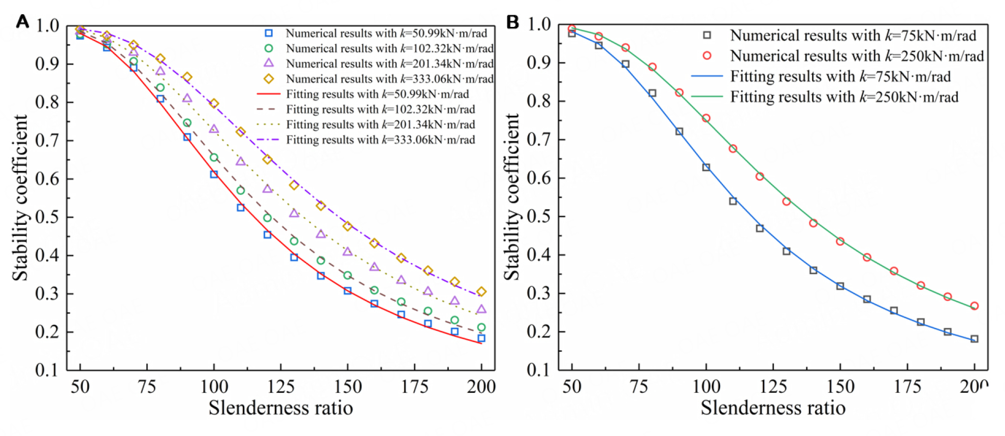
Figure 3. Accuracy validation of proposed fitting formula. (A) Comparison of fitting and numerical results; (B) Prediction by proposed fitting formula.
In STTTs, there are two typical kinds of steel-tube members, namely, the tension-bending and compression-bending members. Tension-bending members that are subjected to the bending moment and axial tension force always exhibit strength failure. Regarding compression-bending members that are subjected to the bending moment and axial compression force, their failure is controlled by their stability behavior. However, in the dynamic analysis, it is slightly impracticable to concentrate on the time-efficiency and mature method for estimating the buckling point for all tower members at all-time steps. Thus, the critical strength approach suggested by design specifications is adopted to determine the dynamic stress of members[5]; i.e., the dynamic stress of steel-tube members is calculated via their stability coefficient.
For compression-bending members, their dynamic stress could be calculated by[22]
where
where
Regarding tension-bending members, due to their failure controlled by their strength, their dynamic stress
STOCHASTIC STRESS RESPONSE ANALYSIS AND DYNAMIC RELIABILITY EVALUATION FOR STTTS CONSIDERING EFFECTS OF SEMI-RIGID CONNECTED JOINTS AND SEMI-RIGID-CONSTRAINED STABILITY BEHAVIORS
In this section, the stochastic dynamic FE model of STTTs with semi-rigid behaviors (STTTs-SRB) is constructed first. Then, by introducing the proposed fitting formula for the stability coefficient of STMs-SRB, the sample set of the stochastic stress response of STTTs considering effects of semi-rigid connected joints and semi-rigid-constrained stability behaviors is determined. Afterward, by solving the integral form of GDEE, the evolution process of the probability density function (PDF) of the stochastic stress response is obtained. Finally, on the basis of the extreme-value distribution method, the dynamic reliability of STTTs considering effects of semi-rigid connected joints and semi-rigid-constrained stability behaviors is evaluated.
Stochastic dynamic FE model of STTTs-SRB under stochastic wind excitations
A transmission tower can be considered as an integrated structural system. Assume that
where
where
Stiffness matrix of STTTs-SRB
The main work for the derivation of the stiffness matrix of STTTs-SRB is to determine the element stiffness matrix of STMs-SRB. Thus, in this subsection, the first step is to determine the element stiffness matrix of STMs-SRB. Then, the global stiffness matrix of STTTs-SRB is assembled by all element stiffness matrices of STMs-SRB.
The element of STMs-SRB is shown in Figure 1, the length of which is
where
In Equations (12)-(14), we have
Mass matrix of STTTs-SRB
As a type of boundary condition, the semi-rigid connection will influence the consistent mass matrix of elements because the consistent mass matrix is derived by the shape function of deformations of elements, and the shape function is related to the boundary condition. The consistent mass matrix of STMs-SRB is derived, which can properly reflect their distributed mass. It is expressed as
where
where
Rayleigh damping matrix of STTTs-SRB
The global damping matrix can be defined as the Rayleigh damping matrix, a combination of the global mass and stiffness matrices, and it is expressed as
where
where
In this paper, the Newmark's method[24] is adopted to solve all samples of stochastic FE equations in the time domain. The Newmark's method will be an unconditionally stable numerical approach if its parameters are appropriately taken. By solving all samples of stochastic FE equations, the corresponding samples of stochastic internal force of STMs-SRB could be determined, and then, the sample set of the stochastic stress response of STMs-SRB can be generated by Equations (5-8). Once the sample set is obtained, the GDEE can be used to conduct the stochastic dynamic response analysis and the reliability evaluation, which are exhibited in the following subsections.
Stochastic stress response analysis of STTTs considering effects of semi-rigid connected joints and semi-rigid-constrained stability behaviors
According to the principle of probability conservation[25], the GDEE for the concerned response
where
Actually, the integral form of the GDEE is equivalent to the differential form of the GDEE in the sense of probability conservation, and the former can deduce the latter[30]. However, it is worth noting that solving the GDEE in the differential form needs the derivative of responses. In this paper, we are concerned about the stress of members, while the derivative of the stress of members may not be easily obtained. Accordingly, due to no need for the derivative of responses, solving the GDEE in the integral form might be a more appropriate way for this paper.
Generally, the analytical solution of the GDEE is hard to obtain owing to the complex behavior of dynamic response and the complexity of mapping. To this end, two techniques are introduced in the GDEE: (1) partition of input probability space; (2) smoothing of Dirac delta function. Based on the Voronoi cell-based partition technique and GF-discrepancy-based point selection strategy[31], the former can reduce the numerical error by generating representative points and assigned probabilities that represent the probability space. The latter aims to improve the integral accuracy by smoothing the integrand, e.g., the Gaussian function. By employing a family of Dirac's sequences[27–29] based on the normal distribution, Equation (22) can be further presented as
where
where
Dynamic reliability evaluation of STTTs considering effects of semi-rigid connected joints and semi-rigid-constrained stability behaviors
Based on the extreme-value distribution method[20], once the critical dynamic response exceeds the safety limit at a time instant, the structure will be considered to have failed. Therefore, the key stochastic dynamic response at each discrete time instant can compose a series system in the time domain
In transmission towers, the stress response of members can be constructed as an extreme-value variable. Further, the performance function of the extreme-value variable can be constructed as
where
where
Implementation procedure
In general, the flowchart of the stochastic stress response analysis and dynamic reliability evaluation of STTTs considering effects of semi-rigid connected joints and semi-rigid-constrained stability behaviors is shown in Figure 4, and the corresponding implementation procedure can be summarized as follows.
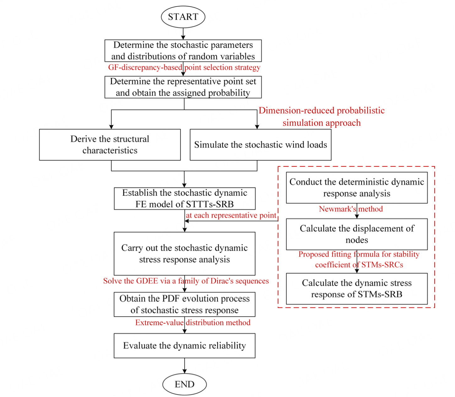
Figure 4. Flowchart of stochastic stress response analysis and dynamic reliability evaluation.
Step 1: Take the random variables of STTTs-SRB (namely, semi-rigid connections, wind loads, dimensions, and materials).
Step 2: Determine the representative point set and obtain its corresponding assigned probability by the GF-discrepancy-based point selection strategy. Step 3: Simulate the stochastic wind loads of STTTs based on the dimension-reduced probabilistic simulation approach.
Step 4: Determine the structural characteristics of STTTs-SRB, including the stiffness, mass, and damping matrices, to construct their stochastic dynamic FE model.
Step 5: Carry out the deterministic dynamic response analysis at each representative point and obtain the sample set of the stochastic stress response.
Step 6: Carry out the stochastic dynamic response analysis by solving the GDEE via a family of Dirac's sequences.
Step 7: Obtain the PDF evolution process of the stochastic stress response of STTTs considering effects of semi-rigid connected joints and semi-rigid-constrained stability behaviors.
Step 8: Evaluate the dynamic reliability of STTTs considering effects of semi-rigid connected joints and semi-rigid-constrained stability behaviors based on the extreme-value distribution method.
ENGINEERING EXAMPLE
Description of the transmission tower
An STTT is adopted to assess its wind-induced dynamic stress. Because of unpredictable computational cost involved in such a complex and huge structural form, it is quite time-consuming to calculate the wind speed for all nodes of transmission towers. Accordingly, for simplification, transmission towers are often properly divided into a number of simulation areas along the tower height, and each simulation area is represented by a point to calculate the wind speed[23,32]. By adopting this way, the employed transmission tower is simplified as nine appropriate simulation points to calculate the wind speed, as illustrated in Figure 5. Some design parameters of the tower and lines are listed in Table 2. It is assumed that the wind direction is perpendicular to the transverse plane, and the span of the employed tower is taken as 500 m.
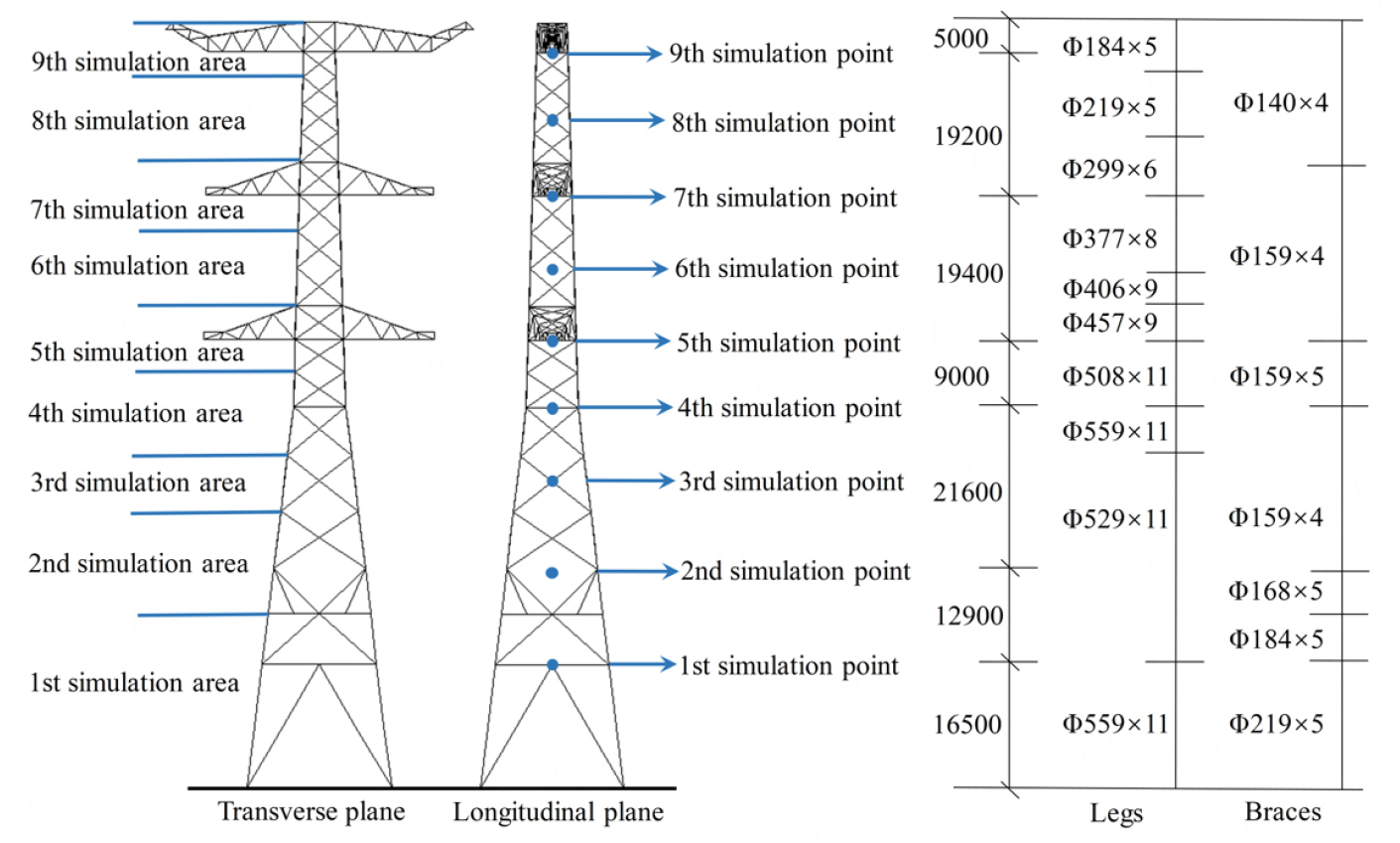
Figure 5. Simulation areas and points of wind loads.
Design parameters of the employed tower and lines
| Design parameters | Type or value | |
| Tower | Height (m) | 103.6 |
| Steel grade | Q355 | |
| Design wind speed (m/s) | 25 | |
| Conductor wire | Outer diameter (mm) | 33.6 |
| Weight (kg/m) | 2.06 | |
| Ground wire | Outer diameter (mm) | 15.75 |
| Weight (kg/m) | 0.99 | |
By determining the stiffness, mass, and damping matrices of the STTT and the wind load vector, its dynamic FE model is established. For better properties of efficiency and fitting actual engineering practice, the gusset plates and bolts of joints are not established in the FE model[14,17,32], and the semi-rigid connections are adopted to represent the joints[23]. It is assumed that the elastic modulus, the Poisson's ratio, and the density of steel material are taken as 206 GPa, 0.3, and 7, 850 kg/
Determination of random variables
Some basic random variables are selected, and their statistical properties are listed in Table 3. Referring to the probabilistic model code[33], the probability distribution of the elastic modulus, Poisson ratio, and yield strength is taken as the lognormal distribution, and the probability distribution of the thickness and outer diameter of steel tube members is taken as the normal distribution. Meanwhile, the probability distribution of the damping ratio is also taken as the normal distribution[34]. In addition, the fluctuating wind speed is simulated as a stochastic process by taking two independent random variables (
Statistical property of basic random variables
| Basic random variables | Symbol | Distribution | Mean | COV |
| COV is the coefficient of variation; | ||||
| Outer diameter | Normal | 0.05[33] | ||
| Thickness | Normal | 0.05[33] | ||
| Damping ratio | Normal | 0.02 | 0.4[34] | |
| Elastic modulus | Lognormal | 2.06 | 0.03[33] | |
| Poisson ratio | Lognormal | 0.3 | 0.03[33] | |
| Yield strength | Lognormal | 387 (MPa) | 0.07[33] | |
| Elementary random variables for wind speed | Uniform | |||
| Uniform | ||||
| Semi-rigid connection | Uniform | 175 (kN | ||
Results of stochastic stress response and dynamic reliability
Generally, the maximum response of structures is the key and concerned response. Accordingly, in this practical example, the maximum member stress in transmission towers is selected to illustrate the results of stochastic stress responses of the STTT considering effects of semi-rigid connected joints and semi-rigid-constrained stability behaviors. The location of the maximum member stress in the transmission tower is shown in Figure 6. Figure 7 shows the PDF evolution process of the maximum member stress of the STTT considering effects of semi-rigid connected joints and semi-rigid-constrained stability behaviors within the time interval from 100 s to 500 s. It can be clearly seen that the evolution process of the PDF surface and contour with the time-variant peak is noticeably non-smooth, which indicates that the stress of members induced by the random variables presents strongly stochastic and time-variant characteristics. Correspondingly, Figure 8 shows the time histories of the mean and standard deviation (STD) of maximum member stress. Similar to Figure 7, the time histories of the mean and STD of maximum member stress are time-variant, in which its mean fluctuates around 100 MPa and STD fluctuates around 40 MPa.
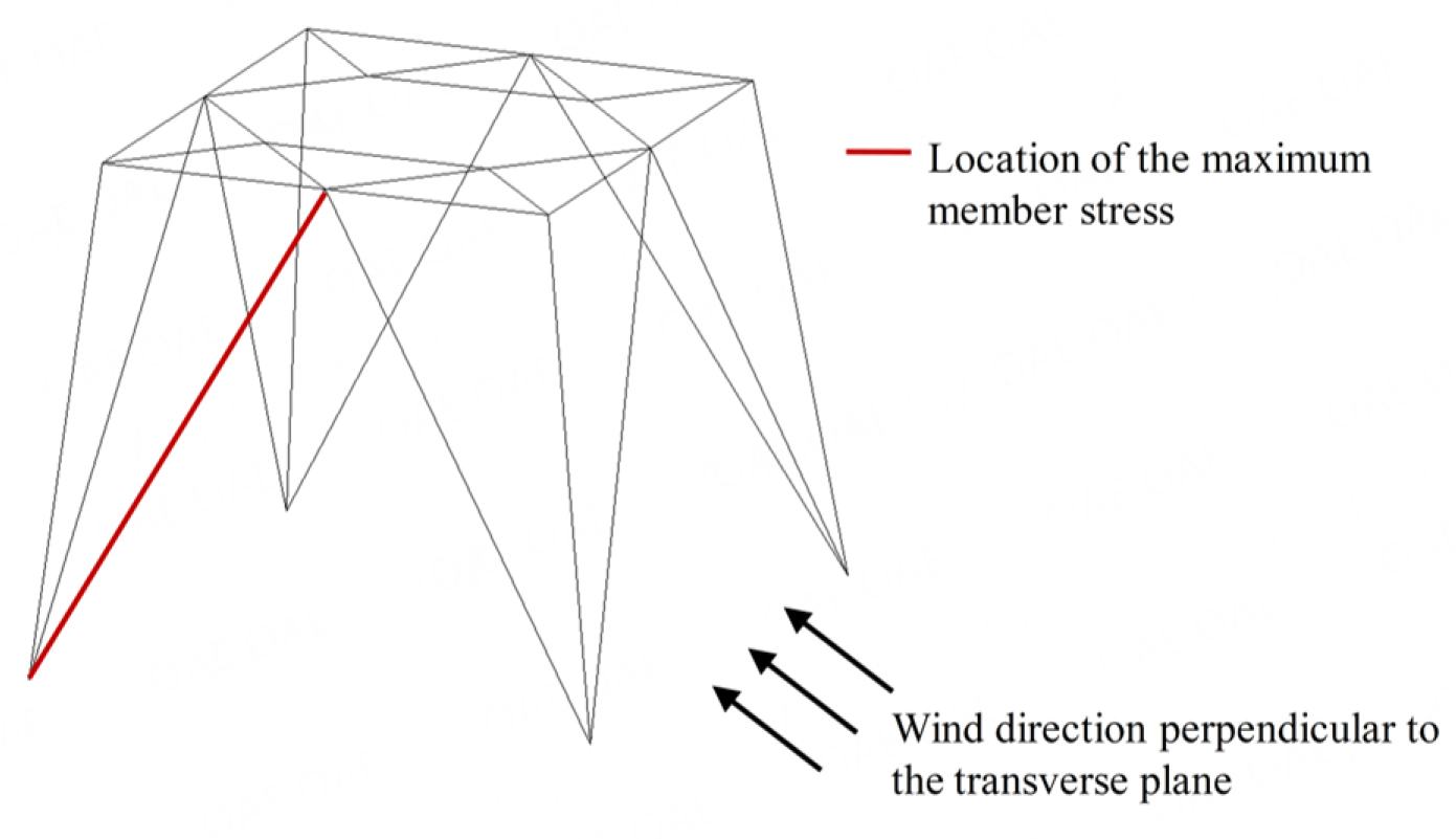
Figure 6. Location of the maximum member stress in the transmission tower.
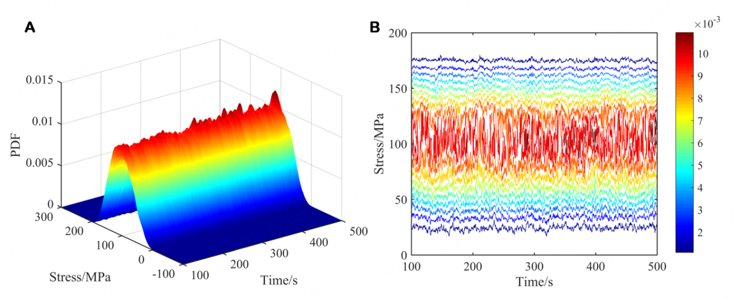
Figure 7. PDF evolution process of maximum member stress within the time interval [100 s-500 s]. (A) The PDF surface; (B) The PDF contour.

Figure 8. Time histories of the mean and STD of maximum member stress. (A) The mean; (B) The STD.
In terms of the dynamic reliability, the reliability index of the STTT considering effects of semi-rigid connected joints and semi-rigid-constrained stability behaviors is calculated as 4.1039 according to the established performance function of extreme-value variables.
Comparisons of analysis results of transmission towers with different connections and stability coefficients
In order to study the effects of semi-rigid connected joints and semi-rigid-constrained stability behaviors on the structural dynamic response and dynamic reliability of transmission towers, the stochastic stress response analyses and reliability evaluations of transmission towers considering pinned and rigid connected joints are also conducted, respectively. It is noted that once the pinned or rigid connected joint is adopted for the transmission tower, the corresponding stability coefficient would change with it. Therefore, in the following subsections, when the different (semi-rigid, rigid, and pinned) connections are adopted, the corresponding stability coefficients are calculated by members with distinct (semi-rigid, rigid, and pinned) connections, respectively.
A sample of stochastic stress response with different connections and stability coefficients
To investigate the effects of semi-rigid connected joints and semi-rigid-constrained stability behaviors on the value of structural responses of transmission towers, the comparisons of a sample of maximum member stress with various connections and stability coefficients are shown in Figure 9. Generally, the variation trend of samples of maximum member stress with rigid and pinned connected joints is basically consistent with that with semi-rigid connected joints. The sample of maximum member stress with semi-rigid connected joints is between that with rigid and pinned connected joints. Table 4 shows the statistical parameters of time-history curves for towers with different connections and stability coefficients, including the mean and STD. Specifically, the mean and STD of time-history curves for the transmission tower considering semi-rigid connected joints are both larger than those considering rigid connected joints while are less than those considering pinned connected joints. This can be explained by the fact that the stress of members is composed of the stress caused by axial forces and bending moments [i.e., Equation (5)]. Although pinned connected joints ignore bending moments, the stability coefficient of members with pinned behaviors is the smallest among the three connection types, leading to the relatively large stress caused by axial forces. On the contrary, rigid connected joints cause the largest bending moments, but the largest stability coefficient of members with rigid behaviors leads to the relatively small stress caused by axial forces. Thus, after comprehensively considering the two parts of the stress, the stress calculated by Equation (5) would present the maximum value for members with pinned behaviors, while that would present the minimum value for members with rigid behaviors, and that would present the median value for members with semi-rigid behaviors.
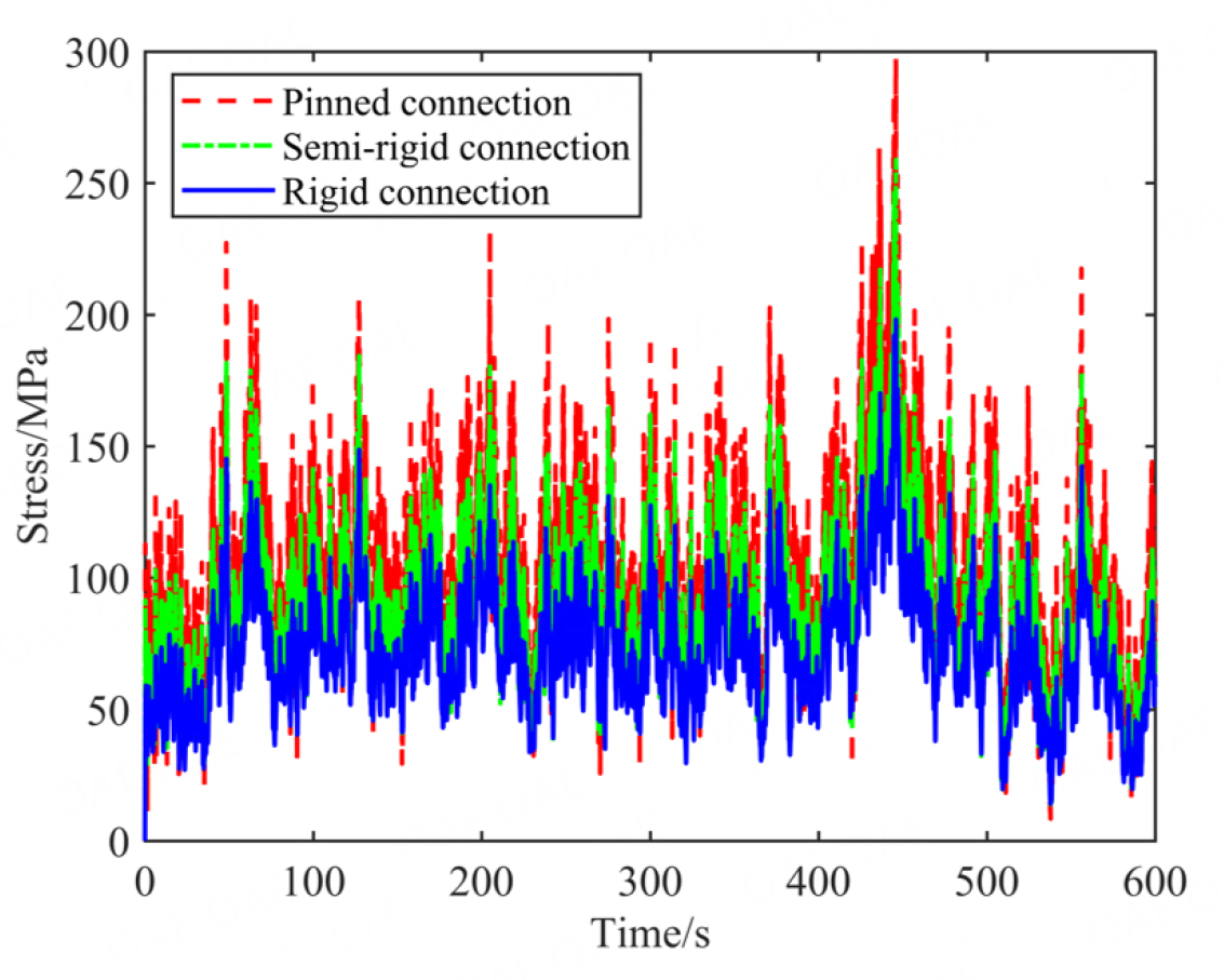
Figure 9. Comparisons of a sample of maximum member stress with different connections and stability coefficients.
Comparisons of mean and STD of time-history curves with different connections and stability coefficients (unit: MPa)
| Rigid connection | Semi-rigid connection | Pinned connection | |
| Mean | 72.7135 | 86.3197 | 101.1282 |
| STD | 23.9091 | 29.3765 | 35.7644 |
| Maximum value | 258.8285 | 86.3197 | 297.2877 |
Stochastic stress response of towers with different stability coefficients and connections
Figure 10 compares the PDF curves of maximum member stress for towers with different stability coefficients and connections at three typical time instants, i.e.,
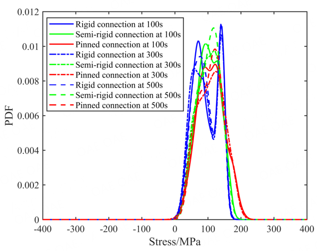
Figure 10. Comparison of PDF for the maximum member stress with different stability coefficients and connections at three typical time instants.
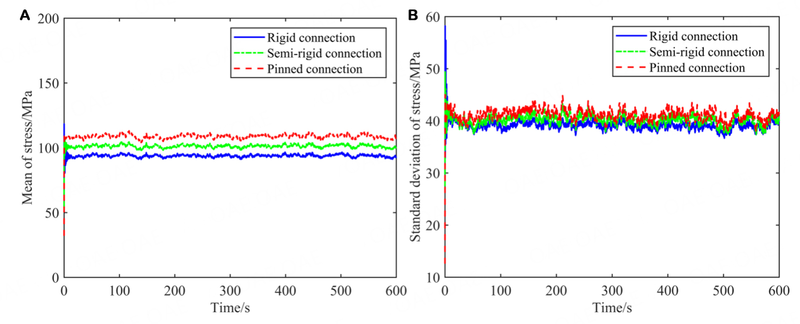
Figure 11. Comparisons of the mean and STD of PDF for maximum member stress with different stability coefficients and connections. (A) The Mean; (B) The STD.
Dynamic reliability of transmission towers with different stability coefficients and connections
The PDF and CDF of the performance function with different stability coefficients and connections are compared in Figure 12. It can be clearly observed that the PDF and CDF curves of the performance function with pinned connected joints are closest to the failure boundary (i.e., 0 MPa), and those with rigid connected joints are farthest from the failure boundary. The PDF and CDF of the performance function with semi-rigid connected joints are between those with pinned and rigid connected joints. Furthermore, the dynamic reliability of transmission towers with different stability coefficients and connections is compared in Table 5. It can be obtained that the reliability index of the transmission tower considering rigid connected joints is calculated as 5.3967 and that considering pinned connected joints is calculated as 3.0304. The reliability index of the transmission tower considering semi-rigid connected joints is smaller than that considering rigid connected joints and is larger than that considering pinned connected joints.

Figure 12. Comparisons of PDF and CDF of the performance function with different stability coefficients and connections. (A) The PDF; (B) The CDF.
Comparisons of reliability indexes for transmission towers with different stability coefficients and connections
| Rigid connection | Semi-rigid connection | Pinned connection | |
| Reliability index | 5.3967 | 4.1039 | 3.0304 |
In summary, the semi-rigid connected joints and semi-rigid-constrained stability behaviors would significantly affect the stochastic stress response and dynamic reliability of STTTs. The time-history curves of the mean and STD of member stress of STTTs considering semi-rigid connected joints and semi-rigid-constrained stability behaviors are between those considering rigid and pinned connected joints and corresponding constrained stability behaviors. Similarly, the dynamic reliability of STTTs considering semi-rigid connected joints and semi-rigid-constrained stability behaviors is smaller than that considering rigid connected joints and rigid-constrained stability behaviors and is larger than that considering pinned connected joints and pinned-constrained stability behaviors. Thus, it is essential to take into account the semi-rigid behavior for STTTs, and the adoption of pinned or rigid behavior in the traditional design and analysis may be inappropriate for these structures.
CONCLUSIONS AND REMARKS
In this paper, a fitting formula is proposed for the stability coefficient of STMs-SRB in transmission towers to determine the dynamic stress. Then, the structural characteristics (namely, stiffness, mass, and damping matrices) of STTTs-SRB are derived to develop its stochastic FE model. Further integrated with the integral form of GDEE and a family of Dirac's sequences, the stochastic stress response analysis is conducted for STTTs considering effects of semi-rigid connected joints and semi-rigid-constrained stability behaviors, and their dynamic reliability is evaluated on the basis of the extreme-value distribution method. Finally, the effects of semi-rigid connected joints and semi-rigid-constrained stability behaviors on the stochastic stress response and dynamic reliability of STTTs are investigated. Some important conclusions and remarks are presented below.
● The proposed fitting formula has the satisfactory accuracy to determine the stability coefficient of STMs-SRB, which can be further used to calculate the dynamic stress response of members in STTTs-SRB.
● The time-history curves of the mean and STD of member stress of STTTs considering semi-rigid connected joints and semi-rigid-constrained stability behaviors are between those considering rigid and connected joints and corresponding constrained stability behaviors.
● The dynamic reliability of STTTs considering semi-rigid connected joints and semi-rigid-constrained stability behaviors is smaller than that considering rigid connected joints and rigid-constrained behaviors and is larger than that considering pinned connected joints and pinned-constrained stability behaviors.
● It is essential to take into account the semi-rigid behavior for STTTs, and the adoption of pinned or rigid behavior in the traditional design and analysis may be inappropriate for these specific tower configurations.
Although this paper investigated the stochastic stress response and dynamic reliability of STTTs considering effects of semi-rigid connected joints and semi-rigid-constrained stability behaviors, there remain some challenges and limitations. This paper aims to assess the stress-based reliability of transmission towers while other limit states (e.g., deformation) are not considered. The reliability of STTTs-SRB considering multiple limit states (strength, stability, and displacement) can be further investigated in future works. In addition, the semi-rigid connections would deteriorate with the increasing service year due to aging, fatigue, chemical corrosion, and physical damage, leading to in-service STTTs further deteriorating over time. Therefore, the prediction model of mechanical properties needs to be established for deteriorating semi-rigid connected joints, and the time-variant reliability evaluation of STTTs also needs to be conducted. It would be helpful to make reasonable maintenance and rehabilitation decisions at an appropriate time for an STTT, which can ensure its satisfactory performance and minimize maintenance costs during its life cycle.
DECLARATIONS
Acknowledgments
The work presented in this paper was fully supported by the Special Support of Chongqing Postdoctoral Research Project (Grant No. 2022CQBSHBT3009) and the Special Postdoctoral Support Project of Chongqing Research Institute of HIT (Grant No. KY506023002). The authors would like to express their gratitude for all the support received
Authors' contributions
Methodology, validation, formal analysis, software, investigation, data curation, visualization, and writing - original draft: Tang ZQ Conceptualization, methodology, software, resources, supervision, and writing - review and editing: Wang T Project administration and writing - review and editing: Li ZL Writing - review and editing: Lu DG, Tan YQ
Availability of data and materials
Some or all data and materials that support the findings of this study are available from the corresponding author upon reasonable request.
Financial support and sponsorship
The research received funding from the Special Support of Chongqing Postdoctoral Research Project (Grant No. 2022CQBSHBT3009) and the Special Postdoctoral Support Project of Chongqing Research Institute of HIT (Grant No. KY506023002).
Conflicts of interest
All authors declared that there are no conflicts of interest.
Ethical approval and consent to participate
Not applicable.
Consent for publication
Not applicable.
Copyright
© The Author(s) 2023.
APPENDIX A: DERIVATION OF CONSISTENT ELEMENT MASS MATRIX OF STMs-SRB
The shape function of the axial displacement
where
Equation (A1) can be expressed in a matrix form as
where
Additionally, the axial displacement vector
where
where
where
Substituting Equations (A1-A3) into Equation (A4) and noting that the bending rotations (
where
According to Equation (A7), the undetermined coefficients are described as
where
Substituting Equation (A9) into Equation (A4), the deformation of STMs-SRB is expressed by the shape functions and nodal displacement as
Considering the boundary condition of steel-tube members, the bending moments (
where
Integrating Equation (A5) with Equation (A12), the rotations of semi-rigid connections (
where
Then, substituting Equation (A13) into Equation (A10), the deflections of STMs-SRB (
where
where
Furthermore, Equation (A18) could be expressed by the nodal displacement vector of elements as
where
where
Finally, the consistent mass matrix of STMs-SRB is determined as
APPENDIX B: EXPRESSIONS OF $$ \bf{H_{zn}} $$ $$ \bf{H_{yn}} $$
In Equations (17)-(19), we have
REFERENCES
1. Savory E, Parke GAR, Zeinoddini M, Toy N, Disney P. Modelling of tornado and microburst-induced wind loading and failure of a lattice transmission tower. Eng Struct 2001;23:365-75.
2. Okamura T, Ohkuma T, Hongo E, Okada H. Wind response analysis of a transmission tower in a mountainous area. J Wind Eng Ind Aerodyn 2003;91:53-63.
3. Battista RC, Rodrigues RS, Pfeil MS. Dynamic behavior and stability of transmission line towers under wind forces. J Wind Eng Ind Aerodyn 2003;91:1051-67.
4. Yang SC, Hong HP. Nonlinear inelastic responses of transmission tower-line system under downburst wind. Eng Struct 2016;123:490-500.
5. Zhang J, Xie Q. Failure analysis of transmission tower subjected to strong wind load. J Constr Steel Res 2019;160:271-9.
6. Shen GH, Cai CS, Sun BN, Lou WJ. Study of dynamic impacts on transmission-line systems attributable to conductor breakage using the finite-element method. J Perform Constr Facil 2011;25:130-7.
7. Li JX, Wang SH, Fu X. Dynamic response of tower-line system induced by insulator breakage considering the collision between the conductor and the ground surface. J Perform Constr Facil 2019;34:04019098.
8. Yin T, Lam HF, Chow HM, Zhu HP. Dynamic reduction-based structural damage detection of transmission tower utilizing ambient vibration data. Eng Struct 2009;31:2009-19.
9. Zhang Q, Fu X, Ren L, Jia ZG. Modal parameters of a transmission tower considering the coupling effects between the tower and lines. Eng Struct 2020;220:110947.
10. Hsu TY, Chien CC, Shiao SY, Chen CC, Chang KC. Analysis of environmental and typhoon effects on modal frequencies of a power transmission tower. Sensors 2020;20:5169.
11. Bhowmik C, Chakraborti P. Analytical and experimental modal analysis of electrical transmission tower to study the dynamic characteristics and behaviors. KSCE J Civ Eng 2020;24:931-42.
12. Fu X, Tan ZX, Li HN, Li G. Static and dynamic response characteristics of a full-scale long-cantilever tower under various loading conditions. J Struct Eng 2023;149:05023002.
13. Zhu YM, Sun Q, Zhao C, Wei ST, Yin Y, Su YH. Operational modal analysis of two typical UHV transmission towers: A comparative study by fast Bayesian FFT method. Eng Struct 2023;277:115425.
14. Zhu YM, Sun Q, Zhao C, Qi H, Su YH. Bayesian operational modal analysis with interactive optimization for model updating of large-size UHV transmission towers. J Struct Eng 2023;149:04023184.
15. Cucuzza R, Rosso MM, Aloisio A, Melchiorre J, Giudice ML, Marano GC. Size and shape optimization of a guyed mast structure under wind, ice, and seismic loading. Appl Sci 2022;12:4875.
16. Li ZL, Hu YJ, Tu X. Wind-induced response and its control of long-span cross-rope suspension transmission line. Appl Sci 2022;12:1488.
17. Liu ZH, Liu ZJ, He CG, Lu HL. Dimension-reduced probabilistic approach of 3-D wind field for wind-induced response analysis of transmission tower. J Wind Eng Ind Aerodyn 2019;190:309-21.
18. Roy S, Kundu CK. State of the art review of wind induced vibration and its control on transmission towers. Structures 2021;29:254-64.
19. Tang ZQ, Li ZL, Wang T. GPR-based prediction and uncertainty quantification for bearing capacity of steel tubular members considering semi-rigid connections in transmission towers. Eng Fail Anal 2022;142:106854.
20. Li J, Chen JB. Stochastic dynamics of structures Singapore: John Wiley & Sons; 2009.
21. Tang ZQ, Li ZL, Wang T. Direct prediction method for semi-rigid behavior of K-joint in transmission towers based on surrogate model. Int J Struct Stab Dyn 2023;23:2350027.
22. National Energy Administration. Technical specification for the design of steel supporting structures of overhead transmission line (DL/T 5486-2020) Beijing: China Planning Press; 2020.
23. Tang ZQ, Li ZL, Wang T, Lu DG, Tan YQ. PDEM-based multi-component and global reliability evaluation framework for steel tubular transmission towers with semi-rigid connections. Eng Struct 2023;295:116838.
24. Li C, Pan HY, Tian L, Bi WZ. Lifetime multi-hazard fragility analysis of transmission towers under earthquake and wind considering wind-induced fatigue effect. Struct Saf 2022;99:102266.
26. Li J, Chen JB. The principle of preservation of probability and the generalized density evolution equation. Struct Saf 2008;30:65-77.
27. Li J, Chen JB. Probability density evolution method for dynamic response analysis of structures with uncertain parameters. Comput Mech 2004;34:400-9.
28. Fan WL, Chen JB, Li J. Solution of generalized density evolution equation via a family of
29. Zhou QY, Fan WL, Li ZL, Ohsaki M. Time-variant system reliability assessment by probability density evolution method. J Eng Mechan 2017;143:04017131.
30. Fan WL, Ang AHS, Li ZL. Reliability assessment of deteriorating structures using Bayesian updated probability density evolution method (PDEM). Struct Saf 2017;65:60-73.
31. Chen GH, Yang DX. Direct probability integral method for stochastic response analysis of static and dynamic structural systems. Comput Meth Appl Mech Eng 2019;357:112612.
32. Chen JB, Yang JY, Li J. A GF-discrepancy for point selection in stochastic seismic response analysis of structures with uncertain parameters. Struct Saf 2016;59:20-31.
33. Joint Committee on Structural Safety (JCSS). Probabilistic model code-part 3-resistance models (JCSS-2001) Denmark: JCSS; 2001.
Cite This Article
Export citation file: BibTeX | RIS
OAE Style
Tang Z, Wang T, Li Z, Lu D, Tan Y. Stochastic stress response and dynamic reliability evaluation for transmission towers with semi-rigid behaviors. Dis Prev Res 2023;2:22. http://dx.doi.org/10.20517/dpr.2023.33
AMA Style
Tang Z, Wang T, Li Z, Lu D, Tan Y. Stochastic stress response and dynamic reliability evaluation for transmission towers with semi-rigid behaviors. Disaster Prevention and Resilience. 2023; 2(4): 22. http://dx.doi.org/10.20517/dpr.2023.33
Chicago/Turabian Style
Tang, Zhengqi, Tao Wang, Zhengliang Li, Dagang Lu, Yiqiu Tan. 2023. "Stochastic stress response and dynamic reliability evaluation for transmission towers with semi-rigid behaviors" Disaster Prevention and Resilience. 2, no.4: 22. http://dx.doi.org/10.20517/dpr.2023.33
ACS Style
Tang, Z.; Wang T.; Li Z.; Lu D.; Tan Y. Stochastic stress response and dynamic reliability evaluation for transmission towers with semi-rigid behaviors. Dis. Prev. Res. 2023, 2, 22. http://dx.doi.org/10.20517/dpr.2023.33
About This Article
Copyright

Data & Comments
Data
0

 Cite This Article 16 clicks

 Like This Article 3
likes
Like This Article 3
likes


Comments
Comments must be written in English. Spam, offensive content, impersonation, and private information will not be permitted. If any comment is reported and identified as inappropriate content by OAE staff, the comment will be removed without notice. If you have any queries or need any help, please contact us at support@oaepublish.com.