Research Article | Open Access | 23 May 2023

Assessment of connectivity reliability and travel time of road networks after earthquake: case study of Aba Autonomous Prefecture

Views: 495 | Downloads: 215 | Cited:

Qiang Dou^1,2,3,4

, ...

Bo-Yi Zhang¹

Dis Prev Res 2023;2:5.

10.20517/dpr.2023.02 | © The Author(s) 2023.

Author Information

Article Notes

Cite This Article

Abstract

The road transportation infrastructure system (RTIS) provides a network of options that support the movement of people and goods. As a critical lifeline system, the resilience assessment of RTISs under the impact of different natural hazards, particularly earthquakes, has attracted extensive attention. When an earthquake occurs, an assessment of the connectivity reliability and travel time on road networks is necessary for emergency planning. In this study, the road network in the Aba Autonomous Prefecture, Sichuan Province, China, was considered as the study area and divided into 13 traffic analysis zones (TAZs) based on the administrative divisions. To consider the uncertainties related to seismic hazard assessment, random fields of ground motions were generated using a Monte Carlo simulation (MCS), considering the spatial correlation. Additionally, a connectivity reliability assessment model and travel time assessment model for the road networks were proposed. The connectivity reliability between the TAZs and increased travel time on the road networks after an earthquake were evaluated using MCS to evaluate the uncertainties related to the damage state assessment of road assets, such as bridges, tunnels, and road segments. Consequently, the results can be used as a theoretical basis for decision-making on the location and number of emergency rescue points after an earthquake and as a functional metric for resilience assessment models.

Keywords

Resilience, road transportation infrastructure system, seismic hazard, connectivity reliability, travel time, Monte Carlo simulation

Download PDF 0 5

INTRODUCTION

The road transportation infrastructure system (RTIS) provides a network of options that support the movement of people and goods^[1]. As a critical lifeline system, the RTIS has attracted extensive attention owing to its resilience under different natural disasters. Among natural disasters, earthquakes pose a great threat to the RTIS^[2,3]. Under the impact of destructive earthquakes, the bridges and tunnels of the RTIS are damaged, which not only leads to the loss in the road traffic capacity but also seriously hinders emergency rescue activities, such as personnel rescue and material delivery. Disruption of the operations of these systems can have cascading effects within the system and on other interconnected critical lifeline systems. In addition to the direct damage to physical transport infrastructure, there may be indirect damage to economic and social systems.

In previous studies, the resilience of an infrastructure system was defined as the joint ability to resist (prevent and withstand) any possible hazards, absorb the initial damage, and recover to normal operation^[4,5]. Cimellaro et al. summarized the resilience of a system into the four points referred to as “4R”: robustness, redundancy, resourcefulness, and rapidity^[6,7]. Bruneau et al. extended the resilience assessment framework to four dimensions: technical, organizational, social, and economic. However, these four dimensions are difficult to realistically quantify using a single performance metric. Furthermore, the performance metrics under consideration are different for different systems^[8]. The relevant theories and empirical studies related to the resilience assessment of the RTIS can generally be grouped into three broad categories: (1) assessment of the RTIS at the component level; (2) assessment of the RTIS at the network level; and (3) emergency management and seismic hazard mitigation of the RTIS.

The component-level resilience assessment is mainly used to study the seismic fragility and functional restoration model of important assets, such as bridges^[9,10] and tunnels^[11,12]. In the United States, a framework was developed using the HAZUS methodology for the fragility assessment of various assets with respect to earthquakes, hurricanes, floods, and tsunamis. Fragility models have been developed for all assets at risk in infrastructure systems, such as utility lifelines and transportation networks^[13]. In Europe, the FP7 SYNER-G project has led to the development of a method for the systemic analysis of interdependent infrastructures (i.e., systems of systems) exposed to seismic hazards using a scenario-based approach. To this end, various fragility models have been reviewed and implemented for all assets at risk to generate failure events and compute the system performance using connectivity- or serviceability-level approaches.

At the network level, different approaches have been adopted for the performance assessment of the RTIS^[14-17]. Different functional metrics, such as connectivity, capacity, and integrated loss estimation, have been applied, depending on the considered time frame, such as the emergency or economic recovery phases^[18]. An overview of the modeling techniques for determining the RTIS performance in disasters is given by Faturechi and Miller-Hooks^[1]. The performance metrics include travel time, flow/capacity, accessibility, topological measures (such as the connectivity), and direct and indirect economic losses. The modeling of possible disasters and associated uncertainties includes specific scenarios, the simulation of a wide range of scenarios, the use of probability distributions, and the identification of the worst-case performance or historical scenarios^[19]. Mathematical models of the system performance are classified into analytical, such as the risk matrix, event tree analysis (ETA), fault tree analysis (FTA), analytical hierarchy process (AHP), simulation (such as through Monte Carlo simulations), or optimization using deterministic or stochastic models. Muriel-Villegas et al. classified the available approaches for investigating the transport network reliability during natural disasters into three main areas: connectivity reliability, performance reliability, and vulnerability^[20]. Moreover, the methods and challenges hindering the modeling and simulation of interconnected infrastructure were discussed by Eusgeld et al.^[21] and Ouyang^[22].

The third category involves research on the emergency management and seismic hazard mitigation of the RTIS. Post-disaster decision-making on recovery management is one of the most promising fields for the application of resilience in engineering practice^[23]. Frangopol and Bocchini proposed an optimization model for the post-disaster restoration schedule of transportation networks with respect to the total present cost, using both the total travel time (TTT) and total travel distance (TTD) as network performance metrics^[24]. In addition to long-term resilience indicators, Karamlou and Bocchini introduced a connectivity-based resilience indicator to optimize the restoration priorities during medium-phase disaster management^[25]. Zhang et al. presented a framework to optimize the restoration schedule of the post-earthquake road network based on the total recovery time (TRT) and the skew of recovery trajectory (SRT)^[26], where the network performance is measured using the weighted average number of reliable interdependent routes over all origin-destination (OD) pairs^[27].

Because seismic hazard and risk assessments have shifted from single structures to spatially distributed infrastructure systems, it is important to generate random fields of ground motion that consider spatial correlations during earthquake risk assessment. The excitations of a seismic event are spatially correlated, and this localized spatial correlation may increase the likelihood of the simultaneous damage of many structures during a seismic event. Recently, many researchers have studied the intra-event spatial correlation of ground motion intensity measures (IMs), such as peak ground acceleration (PGA), peak ground velocity (PGV), spectral acceleration (Sa)^[28-37], and cumulative absolute velocity (CAV)^[38]. Ground motion prediction equations (GMPEs) are important tools used in probabilistic seismic hazard and risk assessments. For a regionally distributed RTIS, a fixed value of the IMs cannot reasonably represent the variation trend in space. Therefore, it is necessary to construct a random field of ground motions with spatial correlations for resilience assessment. Thus, a ground motion influence field was established in this study by considering the spatial correlation of ground motion IMs.

The main contributions of this study are as follows: (1) the impact of uncertainties in both the seismic hazard analysis and asset damage assessment on the connectivity reliability and travel time of RTISs after an earthquake are considered. Here, the spatial distribution maps of the peak ground acceleration (PGA) were generated considering the spatial correlation of ground motions; (2) At the component level, models of the seismic fragility of bridges, tunnels, and road segments are established based on earthquake damage data; (3) at the network level, a framework and methodology for the assessment of the connectivity reliability and travel time are proposed; and (4) The framework and methodology were applied to the road network in Aba Autonomous Prefecture, Sichuan Province, China. Thus, the results can provide a basis for decision-making during the emergency phase after an earthquake.

FRAMEWORK AND METHODOLOGY

The framework of this research study includes five modules, as shown in Figure 1: (1) construction of the road networks of interest for use in the analysis; (2) construction of the random fields of ground motion considering the spatial correlation; (3) simulation of the damage states of road assets, such as bridges, tunnels, and road segments; (4) calculation of the connectivity reliability of the traffic analysis zones (TAZs) after an earthquake using Monte Carlo simulation (MCS); and (5) calculation of the increased travel time on the road networks after an earthquake.

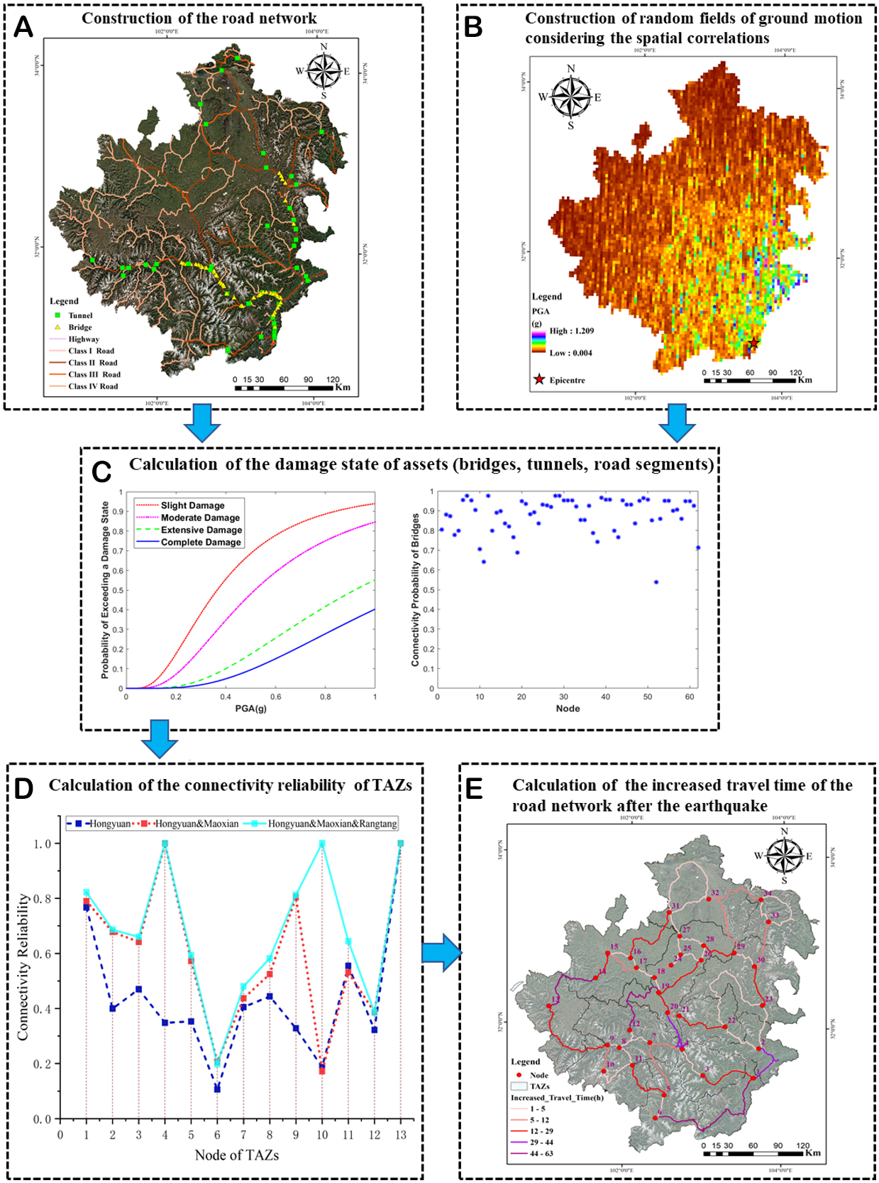
Assessment of connectivity reliability and travel time of road networks after earthquake: case study of Aba Autonomous Prefecture

Figure 1. The framework used in this study: (A) Road network for the case study; (B) PGA values for the study area; (C) Fragility curves and connectivity probability of the road assets; (D) the connectivity reliability of TAZs; (E) The increased travel time on the road network after an earthquake.

Construction of road networks in the study area

The construction of the road networks was achieved through the following steps:

Step 1: Geographic information data for the bridges, tunnels, and road segments were obtained from the China Geographic Information Resource Directory Service System.

Step 2: To ensure the cities remain interconnected within the study area, the road network was simplified according to the road grade and degree of centrality.

Step 3: The cities and road intersections were abstracted as nodes, and the roads between the nodes were abstracted as edges. Each edge consists of a variable number of bridges, tunnels, and road sections, and the relationship between the edges, bridges, tunnels, and road sections was determined using GIS based on their geographical coordinates. Moreover, the properties of the bridges, tunnels, and roadbeds were added to the edges, and a road network model for the evaluation of the network function was developed.

Construction of random fields of ground motion considering the spatial correlations

GMPEs are prediction models used to characterize the variation in the ground motion IMs with factors such as the magnitude, distance, and site. In GMPEs, the randomness of IMs is generally divided into inter-event and intra-event residuals to represent the randomness of the seismic motion intensity measures (IMs). In GMPEs, it is generally assumed that the IMs follow a lognormal distribution. For earthquake event k, the prediction equation of the ground motion intensity parameters of station i at a specific site is:

(1)

$$ \begin{equation} \begin{aligned} \ln \left(Y_{i k}\right)=\ln \bar{Y}_{i k}(M, R, \boldsymbol{\theta})+\eta_{k}+\varepsilon_{i k} \end{aligned} \end{equation} $$

where Y_ik represents the seismic intensity measures at station i when earthquake event k occurs, usually Sa, PGA, PGV, I_a, or other IMs; $$\bar{Y}_{i k}$$(M, R, θ) represents the median value of the ground motion intensity measures estimated by the GMPEs under a given magnitude (M), source distance (R), and other IMs (θ); η_k represents the inter-event residuals for a given earthquake event; η_k is a constant that represents the systematic deviation of the mean value of different seismic events, generally assumed to follow an independent normal distribution with a mean of 0 and standard deviation of σ_η; and ε_ik is the intra-event residuals, which is assumed to follow an independent normal distribution with a mean 0 and a standard deviation of σ_ε.

The standard deviation of the total residual is expressed as σ_T = (σ_η² + σ_ε²)^1/2, and the logarithmic ground motion intensity measures follow a normal distribution:

(2)

$$ \begin{equation} \begin{aligned} \ln \left(Y_{i k}\right) \sim N\left(\ln \bar{Y}_{i k}(M, R, \theta), \sigma_{T}\right) \end{aligned} \end{equation} $$

For the total residual between two random stations i and j at a distance of D in the k-th seismic event, the correlation between η_k(T₁) + ε_ik(T₁) and η_k(T₂) + ε_ik(T₂) can be expressed as:

(3)

$$ \begin{equation} \begin{aligned} \rho_{T}\left(D, T_{1}, T_{2}\right)=\frac{\rho_{\eta}\left(T_{1}, T_{2}\right) \sigma_{\eta}\left(T_{1}\right) \sigma_{\eta}\left(T_{2}\right)+\rho_{\varepsilon}\left(D, T_{1}, T_{2}\right) \sigma_{\varepsilon}\left(T_{1}\right) \sigma_{\varepsilon}\left(T_{2}\right)}{\sigma_{T}\left(T_{1}\right) \sigma_{T}\left(T_{2}\right)} \end{aligned} \end{equation} $$

where T₁ and T₂ are different spectral acceleration periods, ρ_η(T₁, T₂) represents the correlation between the inter-event residuals σ_k(T₁) and σ_k(T₂), and ρ_ε(D, T₁, T₂) represents the correlation between the intra-event residual σ_ik(T₁) and σ_ik(T₂). When T₁ = T₂, ρ_η(T_n, T_n) = 1, the above formula can be simplified to:

(4)

$$ \begin{equation} \begin{aligned} \rho_{T}\left(D, T_{n}\right)=\frac{\sigma_{\eta}\left(T_{n}\right)^{2}+\rho_{\varepsilon}\left(D, T_{n}\right) \sigma_{\varepsilon}\left(T_{n}\right)^{2}}{\sigma_{T}\left(T_{n}\right)^{2}}=\rho_{\eta}\left(T_{n}\right)+\rho_{\varepsilon}\left(D, T_{n}\right) \frac{\sigma_{\varepsilon}\left(T_{n}\right)^{2}}{\sigma_{T}\left(T_{n}\right)^{2}}, \end{aligned} \end{equation} $$

where ρ_η(T_n) represents the inter-event correlation of the ground motion determined using the relationship between the uncertainty components:

(5)

$$ \begin{equation} \begin{aligned} \rho_{\eta}\left(T_{n}\right)=\frac{\sigma_{\eta}\left(T_{n}\right)^{2}}{\sigma_{\eta}\left(T_{n}\right)^{2}+\sigma_{\varepsilon}\left(T_{n}\right)^{2}}=\frac{\sigma_{\eta}\left(T_{n}\right)^{2}}{\sigma_{T}\left(T_{n}\right)^{2}} \end{aligned} \end{equation} $$

The station separation distance Δ_ij is typically calculated using geostatistics. A semi-variogram function, which is a tool function for studying spatial variability in Geo-statistics, was used to characterize the spatial variation structure and spatial continuity of the random variables. It can be expressed as:

(6)

$$ \begin{equation} \begin{aligned} γ(h)=\frac{1}{2N(h)} {\textstyle \sum_{i=1}^{N(h)}}{[V(u_{i}+ h)-V(u_{i})]}^{2} \end{aligned} \end{equation} $$

where h represents the distance between two points in space; γ(h) represents the empirically estimated value of the semi-variogram at distance h, N(h) represents the logarithm of all stations with a distance h between samples; and V(u_i + h) and V(u_i) represent the intra-event residuals of the two stations when the distance is h.

In the case of a given seismic event k and field point i, the seismic motion IM (In(Y_ik)) is a random variable that obeys the normal distribution shown in Equation (1), and the logarithmic median value In$$\bar{Y}_{i k}$$ can be obtained according to the GMPEs. Moreover, the standard deviation of the inter-event residual σ_η and intra-event residual σ_ε can also be obtained; thus, it is necessary to generate residual values that obey normal distributions.

IMs obey not only marginal normal distribution at a given location but also the assumption of multivariate normal distribution at multiple locations. To generate the m-dimensional random field of the total residual of the spatially-correlated earthquake motion IMs, standard normal random variables with a spatial correlation equal to the total residual were first generated, and the multivariate normal vector X = [X₁, X₂, …, X_m]~N_m(0, Σ), where Σ is the correlation coefficient matrix:

(7)

$$ \begin{equation} \begin{aligned} \sum \sim\left(\begin{array}{cccc} 1 & \rho_{12} & \cdots & \rho_{1 m} \\ \rho_{21} & 1 & \cdots & \rho_{2 m} \\ \vdots & \vdots & \vdots & \vdots \\ \rho_{m 1} & \rho_{m 2} & \cdots & 1 \end{array}\right),\\ \end{aligned} \end{equation} $$

where ρ_ij represents the spatial correlation coefficient of different site points calculated according to Equation (5).

In summary, the process of generating a spatially-correlated random field of the total residual values of ground motion at m stations is equivalent to generating a random vector X = [X₁, X₂, …, X_m]. The specific steps were as follows: first, an independent normal vector U = [U₁, U₂, …, U_m] with a mean value of 0 and variance σ_T² was generated, U_m~N(0, σ_T²); second, Cholesky decomposition was performed on the correlation matrix Σ: Σ~BB^T; and finally, a random vector X was obtained using the following formula, where X_j is the total residual error of station j:

(8)

$$ \begin{equation} \begin{aligned} \boldsymbol{X}=\boldsymbol{B} \boldsymbol{U} \end{aligned} \end{equation} $$

Seismic fragility models of the road assets

In this study, seismic fragility models of bridges^[39], tunnels^[11], and road segments^[40] were obtained using the statistics based on the Wenchuan earthquake and other earthquake damage data [Table 1].

Table 1

Median and standard deviation of seismic fragility models

Asset type	Fragility parameters	Slight damage	Moderate damage	Severe damage	Collapse
Bridge	Median (g)	0.3780	0.5346	0.9502	1.2141
Bridge	Log std.	0.6482	0.6482	0.6482	0.6482
Road segment	Median (g)	0.541	0.655	1.243	1.488
Road segment	Log std.	0.774	0.849	0.913	0.501
Tunnel	Fragility parameters	Slight damage	Moderate damage	Severe damage
	Median (g)	0.75	1.28	1.73
	Log std.	0.53	0.53	0.53

Connectivity reliability assessment using the MCS method

The connectivity reliability assessment was performed based on six steps:

Step 1: The PGA value of the sites where bridges, tunnels, and road segments are located in the road network was determined based on their positions.

Step 2: The probability of different road asserts earthquake damage states was simulated based on the seismic fragility models and PGA values.

Step 3: The connectivity probability of each edge was calculated using the following equation:

(9)

$$ \begin{equation} \begin{aligned} P_{e} = P_{b}P_{t}P_{r} \end{aligned} \end{equation} $$

where P_e represents the post-earthquake connectivity probabilities of the edge, and P_b, P_t, and P_r represent the post-earthquake connectivity probabilities of the bridges, tunnels, and subgrades in the edge, respectively.

When calculating the connectivity reliability of the edges based on Equation 9, it was necessary to convert the damage state probability of the assets obtained from the fragility curves into a single connectivity probability value. According to the total probability formula, the connectivity probability of assets was obtained as

(10)

$$ \begin{equation} \begin{aligned} P_{b} \text { or } P_{t} \text { or } P_{r}=\sum_{i=1}^{n} P\left(R \mid D_{i}\right) P\left(D_{i}\right), \end{aligned} \end{equation} $$

where n represents the number of asset damage states, P(D_i) represents the probability that the asset is in a damaged state D_i, and P(R|D_i) represents the probability that the asset is still connected when it is in a damaged state D_i, which is determined by referring to relevant literature^[41].

Step 4: The edge connectivity probabilities were sampled. A k-th sampling simulation was performed to generate the state variable x(k) of the edge, and random numbers r = [r₁, r₂, …, r_n], which are uniformly distributed in the interval [0, 1], were generated.

(11)

$$ \begin{equation} \begin{aligned} x_{i}(k)=\left\{\begin{array}{ll} 1 & r_{i} \leq P_{l i} \\ 0 & r_{i}>P_{l i} \end{array}\right. \end{aligned} \end{equation} $$

where x_i(k) represents the connection state of the i-th edge, and 1 and 0 represent the connected and disconnected states, respectively. Additionally, P_li represents the post-earthquake connectivity probability of the i-th edge.

Step 5: The road network topology of the k-th sampling was determined according to the value of x(k) (deleting the edge of x_i(k) = 0 from the initial road network topology), and the connectivity of TAZs was calculated according to the breadth-first search algorithm.

Step 6: The simulated average connectivity reliability (ACR) among the TAZs was calculated using the following equation:

(12)

$$ \begin{equation} \begin{aligned} \hat{u}=\frac{1}{N} \sum_{i=1}^{N} g(x(k)) \end{aligned} \end{equation} $$

where N represents the number of simulations, and g(x(k)) represents the connection state of the TAZs, wherein 1 represents the connected state and 0 the disconnected state.

Travel time assessment using the MCS method

The travel time assessment was achieved using the following steps:

Step 1: The same as step 1 in the connectivity reliability assessment module.

Step 2: The same as step 2 in the connectivity reliability assessment module.

Step 3: k-th sampling was performed to generate the damage state vectors B(k), T(k), and R(k) of the bridge tunnels and road segments. For the m bridges, the random numbers r = [r₁, r₂, …, r_m] were generated. Based on the fragility function above, the probabilities of different damage states of m bridges were obtained, and the damage states of bridge B_i(k) were determined. Similarly, the T(k) and R(k) of the tunnels and road segments were obtained.

Step 4: Based on Table 2 and the values of vectors B(k), T(k), and R(k), the capacities of the bridges, tunnels, and road segments in the k-th sampling state, and the reduction coefficient vectors f_c(k) and f_v(k) of the bridge tunnels and road segments, were obtained. The values of f_c(e_k) and f_v(e_k) for the edges sampled at the k-th time were obtained by taking the minimum values of f_c(k) and f_v(k) for the assets contained in the edges.

Table 2

Reduction factors for the post-earthquake traffic capacity and free flow speed of bridges, tunnels, and road segments

Asset type	coefficient	Intact	Slight damage	Moderate damage	Severe damage	Collapse
Bridge & road segment	f_c	1.00	0.90	0.60	0.30	0.00
Bridge & road segment	f_v	1.00	0.80	0.60	0.40	0.00
Tunnel	Coefficient	Intact	Slight damage	Moderate damage	Severe damage
	f_c	1.00	0.90	0.50	0.30
	f_v	1.00	0.80	0.50	0.40

Step 5: The simulated mean value of the traffic capacity reduction coefficients (f_c(e)) and free-flow speed reduction coefficients (f_v(e)) of the edge set were calculated using the following equations, respectively:

(13)

$$ \begin{equation} \begin{aligned} f_{\boldsymbol{c}}(\boldsymbol{e})=\frac{1}{N} \sum_{i=1}^{N} f_{\boldsymbol{c}}\left(\boldsymbol{e}_{k}\right) \end{aligned} \end{equation} $$

(14)

$$ \begin{equation} \begin{aligned} f_{\boldsymbol{v}}(\boldsymbol{e})=\frac{1}{N} \sum_{i=1}^{N} f_{\boldsymbol{v}}\left(\boldsymbol{e}_{\boldsymbol{k}}\right) \end{aligned} \end{equation} $$

Based on the f_c(k) and f_v(k) values, the post-earthquake traffic capacity vector C_a*(k) and free-flow time vector t₀*(k) of the edges were calculated according to Table 2.

Step 6: To analyze the road network before and after the earthquake, the travel time was calculated according to the static traffic assignment method. The increase in the travel time on the road network after the earthquake was calculated using the following equation:

(15)

$$ \begin{equation} \begin{aligned} \Delta t=t_{\text {post }}-t_{\text {pre }} \end{aligned} \end{equation} $$

where Δt represents the increased travel time, and t_pre and t_post represent the travel times before and after the earthquake, respectively.

CASE STUDY: ROAD NETWORK IN THE ABA AUTONOMOUS PREFECTURE, SICHUAN PROVINCE

Construction of the road network

The simplified road network in the Aba Autonomous Prefecture, Sichuan Province, is shown in Figure 2A, including 62 bridges, 36 tunnels, and 698 road segments. As shown in Figure 2B, the study area was divided into 13 TAZs according to the administrative division, and the centroids of the 13 TAZs were connected to the road network as nodes. In the road network, from the highway to the class IV road, the traffic capacities are 1,400, 1,200, 1,000, 800, and 600 pcu/h, and the speed is 100, 80, 60, 40, and 30 pcu/h, respectively.

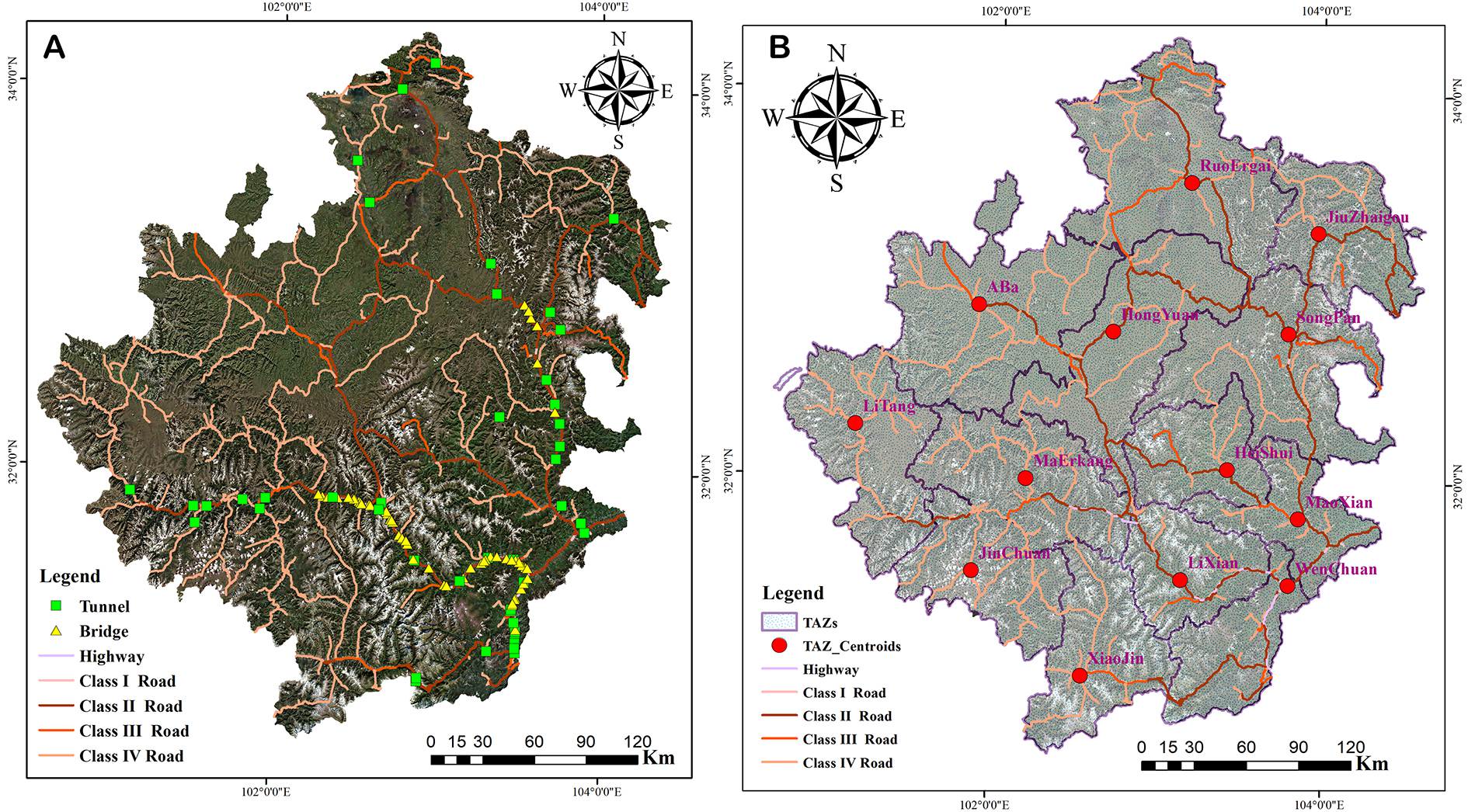
Figure 2. Road network for the case study: (A) location of the bridges, tunnels, and road segments; and (B) division of the TAZs

Construction of random PGA fields considering the spatial correlation

The study area was divided into 1 km × 1 km grids. It was assumed that the faults in this area were normal faults and that the average site condition of the area was bedrock. Additionally, the shear wave velocity was assumed to obey a normal distribution with a mean of 600 m/s and a standard deviation of 50 m/s. 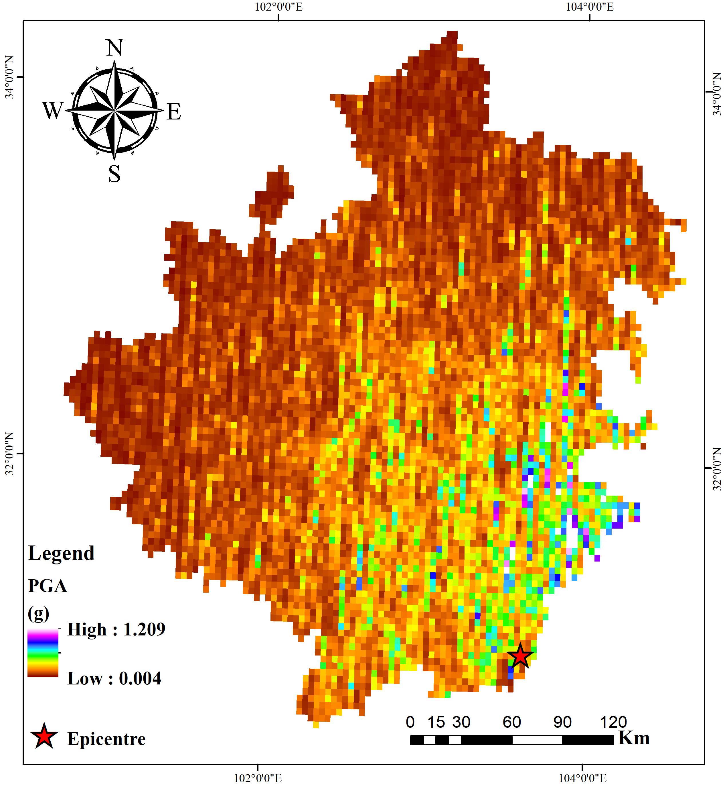There was only one potential focal fault in this area, which only produces earthquakes with a magnitude of M_W = 8.3, an annual average incidence rate of 0.01, and a hypocenter depth of 15 km for a set scenario earthquake event, assuming that the earthquake center is located at 103.42 E and 31.01 N. The CY14 GMPE was used to predict the median value and standard deviation. We conducted 10⁴ MCS to generate the random fields of PGA, considering the spatial correlation. According to the aforementioned conditions, the predicted PGA values for the study area are shown in Figure 3. The values range from 0 to 1.209 g and decrease with an increase in the distance from the earthquake epicenter.

Figure 3. PGA values for the study area.

Simulation of the damage states of the bridges, tunnels, and road segments

The PGA values were extracted according to the positions of the bridges and tunnels and the midpoints of the road segments. As shown in Figure 4, the fragility curves of the bridges [Figure 4A], tunnels [Figure 4B], and road segments [Figure 4C] were obtained according to the aforementioned fragility models.

Figure 4. Fragility curves of the road assets: (A) bridges, (B) tunnels, and (C) road segments.

Connectivity reliability of the edges and network

After calculating the probabilities of different road asset damage states, the connectivity probabilities of the bridge tunnels and road segments were calculated according to Equation 11, as shown in Figures 5 and 6. According to the results obtained from the MCS, the tunnels exhibited the highest connectivity probability (as shown in Figure 5B), with most of them being in the range of 0.9-1. 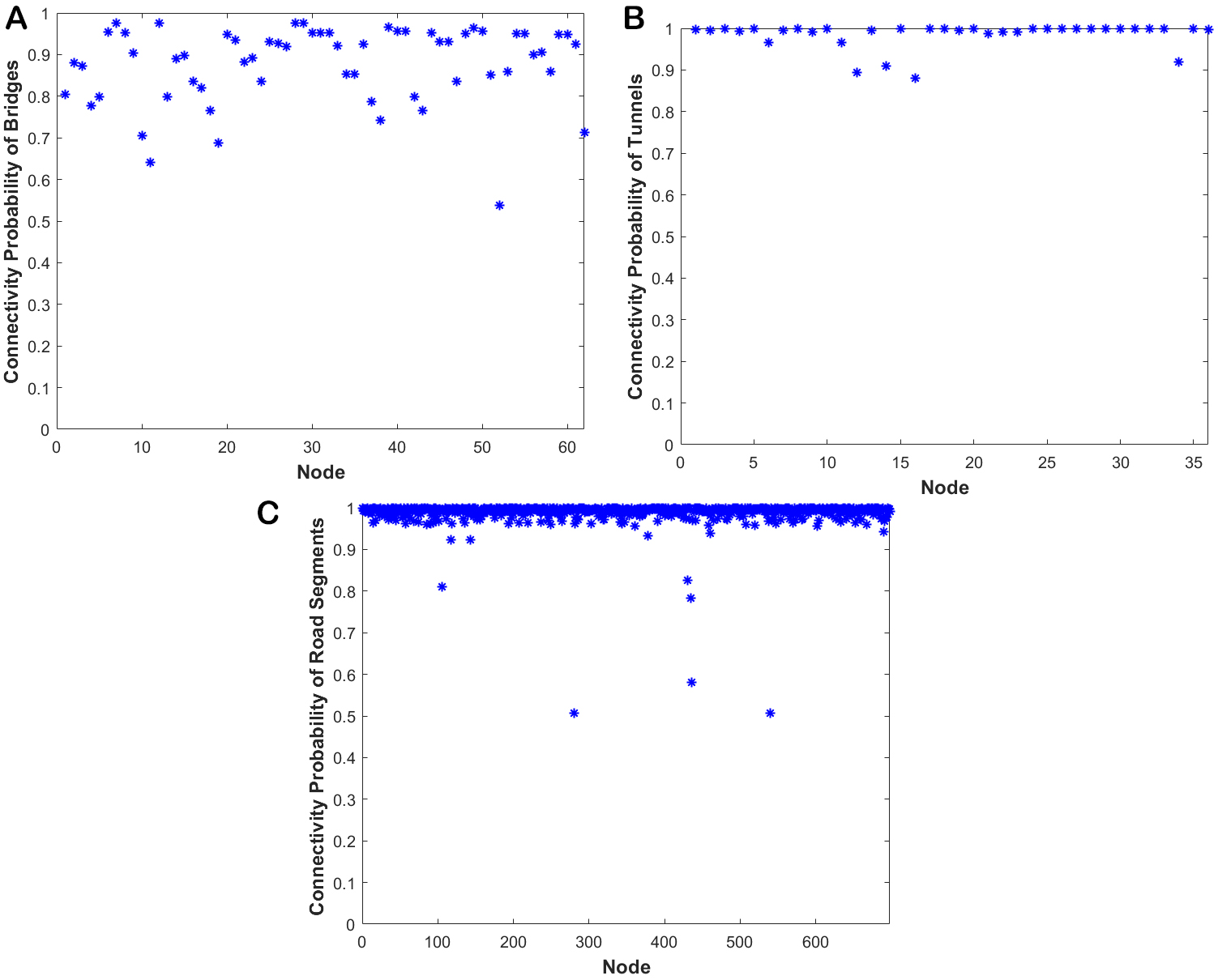Only four hours in the range of 0.8-0.9. Moreover, the connectivity probability of the road segments (as shown in Figure 5C) is mostly in the range of 0.9-1, with only six having a connectivity probability in the range of 0.4-0.9. The connection probability of the bridges [Figure 5A] was relatively low, with a distribution range of 0.5-1. Therefore, the connectivity reliability of the edge was found to be higher for the bridges.

Figure 5. Connectivity probability of the road assets: (A) bridges, (B) tunnels, and (C) road segments.

Figure 6. The visualization of connectivity probability of road assets in GIS.

The connectivity reliability of the edges can be obtained from the results of the asset connectivity probability. In this study, the centroids 1, 2, and 3 of the TAZs were selected as the source points for analyzing the connectivity reliability between the centroids of the 13 TAZs in the study area. We calculated all the combinations of these three source points. Moreover, for the determination of the connectivity between the source points and other centroids when two or three TAZs are selected as source points, we consider other centroids to be connected when they were connected to one of the source points.

For all combinations, which comprise one, two, and three TAZs, we conducted 10⁴ MCS, and the average connectivity reliability (ACR) was calculated. The nodes and names of TAZs are shown in Table 3. As shown in Figure 7, when one TAZ is selected as the source point, the Hongyuan TAZ has the highest ACR among the TAZs, and when two TAZs are selected as the source points, the Hongyuan and Maoxian TAZs have the highest ACR. A comparison of the ACRs shows that the highest ACR of two TAZs is 11.7% higher than that of the single TAZ. Moreover, when three TAZs are selected as source points, the Hongyuan, Maoxian, and Rangtang TAZs have the highest ACR, and the highest ACR of the three TAZs is only 2% higher than that of the two TAZs. In the earthquake scenario assumed in this study, two emergency rescue points were set up in the study area after the earthquake, at Hongyuan and Maoxian.

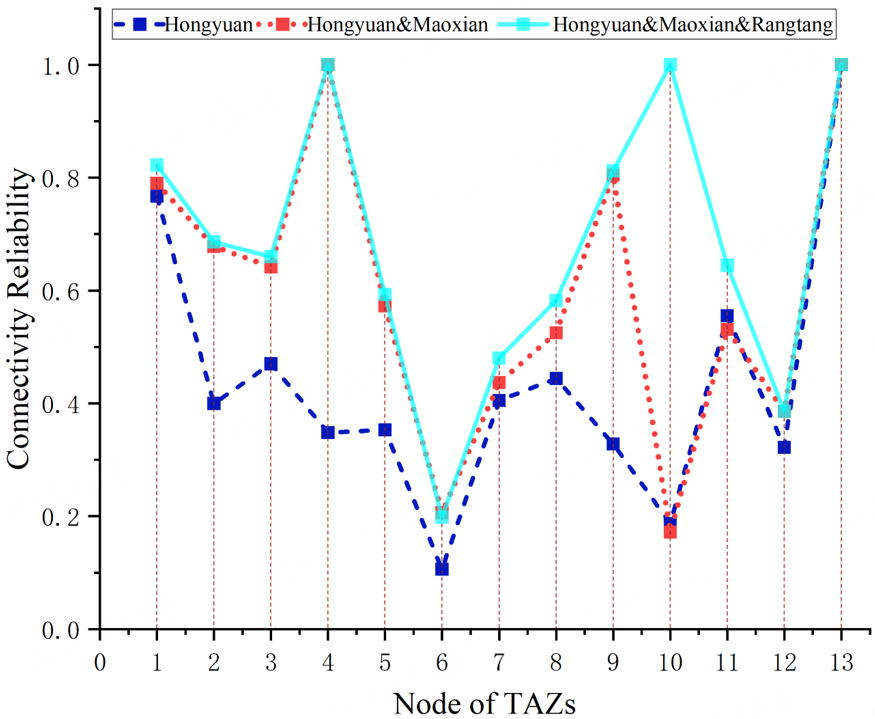
Figure 7. Connectivity reliability of the TAZs.

Table 3

The nodes and names of TAZs

Node	1	2	3	4	5
Name	Maerkang	Wenchuan	Lixian	Maoxian	Songpan
Node	6	7	8	9	10
Name	Jiuzhaigou	Jinchuan	Xiaojin	Heishui	Rangtang
Node	11	12	13
Name	Aba	Ruoergai	Hongyuan

Simulation of the travel time on the road network

Regarding the simulation of the travel time, this study was based on the following assumptions.

1. Owing to the lack of OD matrices in the 13 TAZs, the OD matrices used in this study were based on the population proportion of the TAZs.

2. The traffic demand before and after the earthquake remains the same.

The traffic flow and travel time of each edge were simulated according to the road network OD matrices and traffic capacity of the edge before and after the earthquake. We conducted 10⁴ MCS and calculated the increased travel time according to Equation 16, and the results are shown in Figure 8. The increased travel time is distributed between 1 h and 63 h, and edges with travel time exceeding 12 h are widely distributed throughout the study area. Therefore, earthquakes have a significant impact on the road network travel time. Additionally, the total travel time (TTT) and travel time delay (TTD) are important functional metrics for road network resilience assessment. Based on the aforementioned results, the travel time assessment model based on the MCS method proposed in this study can be used as a foundation for the development of road network resilience assessments.

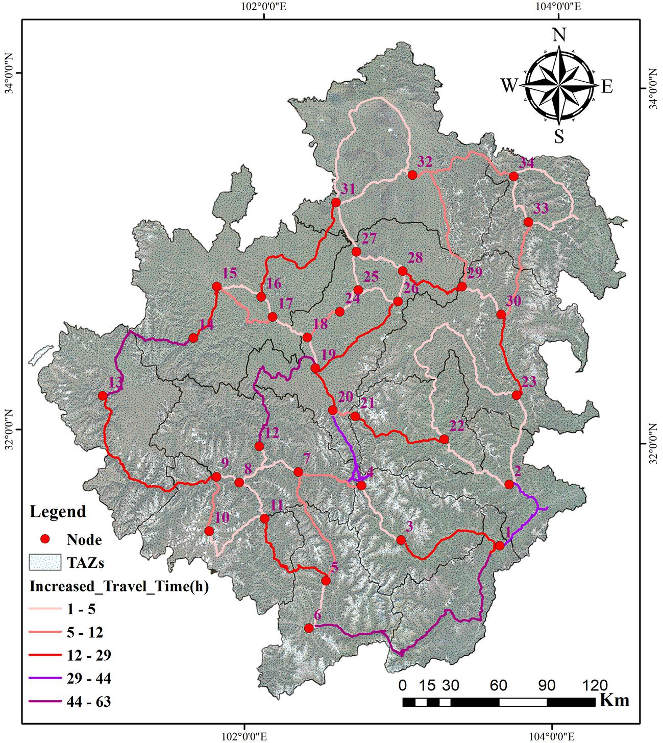
Figure 8. The increased travel time of the road network after an earthquake.

CONCLUSIONS

In this study, the functional metrics of road networks during earthquakes were investigated. To account for the impact of uncertainty in seismic hazard analysis and highway asset damage assessment, a distribution map of the seismic intensity parameters was generated considering the spatial correlation of ground motions. An assessment framework and methodology of the connectivity reliability and travel time using MCS were also proposed. The framework and methodology were then applied to the road network in Aba Autonomous Prefecture, Sichuan Province, China. Consequently, the following were the main conclusions:

(1) In a large-scale distribution area, the intensity of ground motions has a significant effect on the spatial correlation changes. Considering the spatial correlation, the PGA distribution changes more uniformly, which is more in line with the spatial distribution characteristics of real IMs.

(2) When two TAZs were selected as source points, the Hongyuan and Maoxian TAZs had the highest ACR, and the highest ACR of the two TAZs was 11.7% higher than that of a single TAZ. When three TAZs were selected as source points, the Hongyuan, Maoxian, and Rangtang TAZs had the highest ACR, and the highest ACR of the three TAZs was only 2% higher than that of the two TAZs. In the earthquake scenario assumed in this study, two emergency rescue points were set up in the study area after the earthquake, at Hongyuan and Maoxian. Therefore, the connectivity reliability model proposed in this study can provide a theoretical basis for decisions on the number and location of emergency rescue points after an earthquake.

(3) The increased travel time of the edges is distributed between 1 h and 63 h, and edges exceeding 12 h are widely distributed in the study area. This shows that earthquakes have a significant impact on the road network travel time. Moreover, the total travel time (TTT) and travel time delay (TTD) are important functional metrics for road network resilience assessment. Therefore, the proposed travel time assessment model based on the MCS method can be used as a foundation for the development of road network resilience assessments.

DISCUSSION

Resilience assessment is probabilistic in nature; therefore, uncertainty needs to be integrated into all the steps of resilience evaluation, including the modeling of hazard events, response of exposed road infrastructures, and evaluation of functional losses.

The spatial correlation of the ground motion field generated by the GMPEs was built using a correlation distance and intra-event variability. It is an essential component of the seismic risk analysis of RTISs. In contrast to the GMPE used in most current studies to construct earthquake scenarios, the spatial correlation of the ground motion was considered in this study. Compared with the PGA ShakeMap without spatial correlation, the intensity distribution of the PGA ShakeMap with spatial correlation is more uniform and consistent with the attenuation characteristics of the real spatial distribution of the ground shaking intensity parameters. In future research, more uncertainty issues should be considered in seismic hazard assessment, such as the estimation of design earthquake events, occurrence of earthquake events, choice of GMPEs, and estimation of the site amplification factor for a specific site.

Once various sources of uncertainty have been identified, they must be associated with a set of probabilistic distributions. The variability of uncertain sources can be expressed in several ways. An MCS method consists of the sampling of random realizations of various input variables, and the estimation of the final risk metric for each run can be used. After many runs, a stable estimation of the probabilistic distribution of the outcome can be constructed. Even though it is straightforward in principle, the MCS method may require an almost intractable number of runs to achieve convergence, especially when extreme risk values (low probability outcomes) have to be sampled. However, robustness to the number of input variables (high dimensionality) is one of the main merits of MCS methods. In this study, the sampling of the damage states of bridges, tunnels, and road segments was implemented based on the MCS method. Subsequently, the connectivity reliability and travel time were analyzed based on the simulation results and were found to be closer to the actual damage scenario.

This study can be further improved by using a more accurate OD matrix and a dynamic traffic assignment (DTA) model. Moreover, the change in the traffic demand before and after the earthquake and the uncertainty of the division of bridges, tunnels, and subgrade damage states can also be considered.

DECLARATIONS

Authors’ contributions

Substantial contributions to conception and design of the study and performed data analysis and interpretation: Lu DG, Dou Q, Zhang BY

Software, investigation, data curation, methodology, writing-original draft, visualization: Dou Q, Ding JW

Performed technical support: Ding JW, Zhao H

Availability of data and materials

Some or all data and materials that support the findings of this study are available from the corresponding author upon reasonable request.

Financial support and sponsorship

This work was supported by the National Key R&D Program of China (Grant No. 2021YFB2600500) and the Natural Science Foundation of Chongqing CSTC (Grant No. 2022NSCQ-MSX4037).

Conflicts of interest

All authors have declared that there are no conflicts of interest.

Ethical approval and consent to participate

Not applicable.

Consent for publication

Not applicable.

REFERENCES

1. Faturechi R, Miller-hooks E. Measuring the performance of transportation infrastructure systems in disasters: a comprehensive review. J Infrastruct Syst 2015;21:04014025.

2. Tao W, Lin P, Wang N. Optimum life-cycle maintenance strategies of deteriorating highway bridges subject to seismic hazard by a hybrid Markov decision process model. Struct Saf 2021;89:102042.

3. Tao W, Wang N, Ellingwood B, Nicholson C. Enhancing bridge performance following earthquakes using Markov decision process. Struct Infrastruct Eng 2021;17:62-73.

4. Ouyang M, Wang Z. Resilience assessment of interdependent infrastructure systems: with a focus on joint restoration modeling and analysis. Reliab Eng Syst Safe 2015;141:74-82.

5. Liu W, Song Z, Ouyang M, Li J. Recovery-based seismic resilience enhancement strategies of water distribution networks. Reliab Eng Syst Safe 2020;203:107088.

6. Cimellaro GP, Reinhorn AM, Bruneau M. Framework for analytical quantification of disaster resilience. Eng Struct 2010;32:3639-49.

7. Cimellaro GP, Reinhorn AM, Bruneau M. Seismic resilience of a hospital system. Struct Infrastruct Eng 2010;6:127-44.

8. Bruneau M, Reinhorn A. Exploring the concept of seismic resilience for acute care facilities. Earthq Spectra 2007;23:41-62.

9. Aygün B, Dueñas-osorio L, Padgett JE, Desroches R. Efficient longitudinal seismic fragility assessment of a multispan continuous steel bridge on liquefiable soils. J Bridge Eng 2011;16:93-107.

10. Brandenberg SJ, Kashighandi P, Zhang J, Huo Y, Zhao M. Fragility functions for bridges in liquefaction-induced lateral spreads. Earthq Spectra 2011;27:683-717.

11. Argyroudis S, Pitilakis K. Seismic fragility curves of shallow tunnels in alluvial deposits. Soil Dyn Earthq Eng 2012;35:1-12.

12. Avanaki M, Hoseini A, Vahdani S, de Santos C, de la Fuente A. Seismic fragility curves for vulnerability assessment of steel fiber reinforced concrete segmental tunnel linings. Tunn Undergr Space Technol 2018;78:259-74.

13. Neighbors CJ, Cochran ES, Caras Y, Noriega GR. Sensitivity analysis of FEMA HAZUS earthquake model: case study from king county, Washington. Nat Hazards Rev 2013;14:134-46.

14. Noy I, Yonson R. Economic Vulnerability and resilience to natural hazards: a survey of concepts and measurements. Sustainability 2018;10:2850.

15. Attoh-okine NO, Cooper AT, Mensah SA. Formulation of resilience index of urban infrastructure using belief functions. IEEE Syst J 2009;3:147-53.

16. Dong Y, Frangopol DM, Saydam D. Time-variant sustainability assessment of seismically vulnerable bridges subjected to multiple hazards. Earthq Eng Struct Dyn 2013;42:1451-67.

17. Liu C, Ouyang M, Mao Z, Xu X. A multi-perspective framework for seismic retrofit optimization of urban infrastructure systems. Earthq Eng Struct Dyn 2022;51:2771-90.

18. Argyroudis SA, Mitoulis SΑ, Winter MG, Kaynia AM. Fragility of transport assets exposed to multiple hazards: state-of-the-art review toward infrastructural resilience. Reliab Eng Syst Safe 2019;191:106567.

19. Khademi N, Balaei B, Shahri M, et al. Transportation network vulnerability analysis for the case of a catastrophic earthquake. Int J Disaster Risk Reduct 2015;12:234-54.

20. Muriel-villegas JE, Alvarez-uribe KC, Patiño-rodríguez CE, Villegas JG. Analysis of transportation networks subject to natural hazards - insights from a Colombian case. Reliab Eng Syst Safe 2016;152:151-65.

21. Eusgeld I, Nan C, Dietz S. “System-of-systems” approach for interdependent critical infrastructures. Reliab Eng Syst Safe 2011;96:679-86.

22. Ouyang M. Review on modeling and simulation of interdependent critical infrastructure systems. Reliab Eng Syst Safe 2014;121:43-60.

23. Bocchini P, Frangopol DM. Restoration of bridge networks after an earthquake: multicriteria intervention optimization. Earthq Spectra 2012;28:427-55.

24. Frangopol DM, Bocchini P. Resilience as optimization criterion for the rehabilitation of bridges belonging to a transportation network subject to earthquake. Struct Congr 2011:2011;2044-55.

25. Karamlou A, Bocchini P. Sequencing algorithm with multiple-input genetic operators: application to disaster resilience. Eng Struct 2016;117:591-602.

26. Zhang W, Wang N, Nicholson C. Resilience-based post-disaster recovery strategies for road-bridge networks. Struct Infrastruct Eng 2017;13:1404-13.

27. Guidotti R, Gardoni P, Chen Y. Network reliability analysis with link and nodal weights and auxiliary nodes. Struct Saf 2017;65:12-26.

28. Boore DM. Estimated ground motion from the 1994 northridge, california, earthquake at the site of the interstate 10 and la cienega boulevard bridge collapse, West Los Angeles, California. Bull Seismol Soc Am 2003;93:2737-51.

29. Wang M, Takada T. Macrospatial correlation model of seismic ground motions. Earthq Spectra 2005;21:1137-56.

30. Goda K, Hong HP. Spatial correlation of peak ground motions and response spectra. Bull Seismol Soc Am 2008;98:354-65.

31. Jayaram N, Baker JW. Correlation model for spatially distributed ground-motion intensities. Earthq Eng Struct Dyn 2009;38:1687-708.

32. Goda K, Atkinson GM. Intraevent spatial correlation of ground-motion parameters using SK-net data. Bull Seismol Soc Am 2010;100:3055-67.

33. Sokolov V, Wenzel F, Jean W, Wen K. Uncertainty and spatial correlation of earthquake ground motion in Taiwan. Terr Atmos Ocean Sci 2010;21:905.

34. Sokolov V, Wenzel F, Wen K, Jean W. On the influence of site conditions and earthquake magnitude on ground-motion within-earthquake correlation: analysis of PGA data from TSMIP (Taiwan) network. Bull Earthquake Eng 2012;10:1401-29.

35. Esposito S, Iervolino I. PGA and PGV spatial correlation models based on European multievent datasets. Bull Seismol Soc Am 2011;101:2532-41.

36. Esposito S, Iervolino I. Spatial correlation of spectral acceleration in European data. Bull Seismol Soc Am 2012;102:2781-8.

37. Chen Y, Baker JW. Spatial correlations in cyber shake physics-based ground-motion simulations. Bull Seismol Soc Am 2019;109:2447-58.

38. Du W, Wang G. Intra-event spatial correlations for cumulative absolute velocity, arias intensity, and spectral accelerations based on regional site conditions. Bull Seismol Soc Am 2013;103:1117-29.

39. Chen LB, Zheng KF, Zhuang WL, Ma HS, Zhang JJ. Analytical investigation of bridge seismic vulnerability in wenchuan earthquake. J Southwest Jiaotong University 2012;47:558-66.

40. Zhang J, Qu H, Liao Y, Ma Y. Seismic damage of earth structures of road engineering in the 2008 Wenchuan earthquake. Environ Earth Sci 2012;65:987-93.

41. Chang L, Peng F, Ouyang Y, Elnashai AS, Spencer BF. Bridge seismic retrofit program planning to maximize postearthquake transportation network capacity. J Infrastruct Syst 2012;18:75-88.

Cite This Article

Export citation file: BibTeX | RIS

OAE Style

Dou Q, Ding JW, Lu DG, Zhao H, Zhang BY. Assessment of connectivity reliability and travel time of road networks after earthquake: case study of Aba Autonomous Prefecture. Dis Prev Res 2023;2:5. http://dx.doi.org/10.20517/dpr.2023.02

AMA Style

Dou Q, Ding JW, Lu DG, Zhao H, Zhang BY. Assessment of connectivity reliability and travel time of road networks after earthquake: case study of Aba Autonomous Prefecture. Disaster Prevention and Resilience. 2023; 2(2): 5. http://dx.doi.org/10.20517/dpr.2023.02

Chicago/Turabian Style

Dou, Qiang, Jia-Wei Ding, Da-Gang Lu, Hu Zhao, Bo-Yi Zhang. 2023. "Assessment of connectivity reliability and travel time of road networks after earthquake: case study of Aba Autonomous Prefecture" Disaster Prevention and Resilience. 2, no.2: 5. http://dx.doi.org/10.20517/dpr.2023.02

ACS Style

Dou, Q.; Ding J.W.; Lu D.G.; Zhao H.; Zhang B.Y. Assessment of connectivity reliability and travel time of road networks after earthquake: case study of Aba Autonomous Prefecture. Dis. Prev. Res. 2023, 2, 5. http://dx.doi.org/10.20517/dpr.2023.02

About This Article

Special Issue

This article belongs to the Special Issue Recent Progress on Integrated Resilience Testbed Studies

Copyright

© The Author(s) 2023. Open Access This article is licensed under a Creative Commons Attribution 4.0 International License (https://creativecommons.org/licenses/by/4.0/), which permits unrestricted use, sharing, adaptation, distribution and reproduction in any medium or format, for any purpose, even commercially, as long as you give appropriate credit to the original author(s) and the source, provide a link to the Creative Commons license, and indicate if changes were made.

Data & Comments

Data

Views

495

Downloads

215

Citations

Comments

Comments

Comments must be written in English. Spam, offensive content, impersonation, and private information will not be permitted. If any comment is reported and identified as inappropriate content by OAE staff, the comment will be removed without notice. If you have any queries or need any help, please contact us at support@oaepublish.com.