Download PDF
Research Article  |  Open Access  |  19 May 2022

Unconditional and conditional simulation of nonstationary and non-Gaussian vector and field with prescribed marginal and correlation by using iteratively matched correlation

Views: 3053 |  Downloads: 1787 |  Cited:   2
Dis Prev Res 2022;1:5.
10.20517/dpr.2022.01 |  © The Author(s) 2022.
Author Information
Article Notes
Cite This Article

Abstract

In many probabilistic analysis problems, the homogeneous/nonhomogeneous non-Gaussian field is represented as a mapped Gaussian field based on the Nataf translation system. We propose a new sample-based iterative procedure to estimate the underlying Gaussian correlation for homogeneous/nonhomogeneous non-Gaussian vector or field. The numerical procedure takes advantage that the range of feasible correlation coefficients for non-Gaussian random variables is bounded if the translation system is adopted. The estimated underlying Gaussian correlation is then employed for unconditional as well as conditional simulation of the non-Gaussian vector or field according to the theory of the translation process. We then present the steps for augmenting the simulated non-Gaussian field through the Karhunen-Loeve expansion for a refined discretized grid of the field. In addition, the steps to extend the procedure described in the previous section to the multi-dimensional field are highlighted. The application of the proposed algorithms is presented through numerical examples.

Keywords

Simulation, unconditional simulation, conditional simulation, homogeneous and nonhomogeneous non-Gaussian vector or field

1. INTRODUCTION

Probabilistic analysis and reliability estimation often require the unconditional and conditional simulation of the correlated non-Gaussian vector of random variables with the prescribed marginal probability distribution and correlation coefficients. The use of the simulated samples for uncertain propagation or reliability analysis for civil engineering problems is well illustrated in several textbooks[1-3]. The simulation could be carried out by modeling the random variables using the Nataf translation system (or theory of translation process or normal to anything)[3-6], which represents the joint probability distribution of the vector of random variables by the Gaussian copula[7] and probability transformation. The simulation can also be based on normal polynomials[8-11]. A key component of the modeling is to evaluate underlying Gaussian correlation coefficients based on the prescribed correlation coefficients for the non-Gaussian random variables[12-15]. This underlying Gaussian correlation is governed by a double integral equation. Since the analytical solution for the underlying Gaussian correlation is only available under very special circumstances, the underlying characteristics are frequently evaluated using an iterative procedure and numerical integration methods. Moreover, given a correlation coefficient for the non-Gaussian random variables, there is no guarantee that one can find the underlying Gaussian correlation based on the Nataf translation system[12, 13, 16]. An additional problem for the modeling that needs to be dealt with is that the nearest correlation matrix[17, 18] may need to be employed since there is no guarantee that the derived underlying Gaussian correlation matrix from the translation process is positive semi-definite.

Besides simulating the non-Gaussian vector of random variables, the simulation of nonstationary/nonhomogeneous and non-Gaussian random fields is also of importance for structural reliability estimation[19]. Two popular methods to simulate the random field are the spectral representation method (SRM) and the method based on the Karhunen-Loeve (KL) expansion. SRM[20-22] is based on the spectral characteristics of the random field in the time domain, space domain, or both. The spectral characteristics of the field are defined by the power spectral density (PSD) function obtained by using Fourier transform. SRM was extended to simulate nonstationary/nonhomogeneous and non-Gaussian fields[5, 23-26]. These studies use iterative procedures to find the underlying Gaussian PSD function; the PSD and autocorrelation (AC) function forms a Fourier pair (i.e., Wiener - Khintchine theorem). The sampled Gaussian field using the underlying Gaussian PSD function can then be mapped to the non-Gaussian domain based on the theory of the translation process. SRM was extended for conditional simulation in several studies[27-30] for stationary/nonstationary processes and fields based on the conditional joined Gaussian distribution function.

The KL expansion is a special case of the orthogonal series expansion[31]. The orthogonal functions in KL expansion are obtained from the eigenfunctions of a Fredholm integral equation of the second kind with the autocovariance function as the kernel[19]. A random field is represented by the KL expansion with random coefficients. There are many studies focused on simulating the random field based on the KL expansion with engineering applications[19, 32-36]. Since the sum of the KL expansion with random coefficients leads to the Gaussian process, an iterative procedure was proposed[32, 33] to simulate the non-Gaussian process. It includes sampling many sets of random fields, and updating the simulated fields by modifying and shuffling random expansion coefficients based on ranking in each iteration. The adequacy of the sampled field is judged based on the closeness between the marginal distribution of the sampled field and its prescribed distribution. The use of numerical integration to evaluate the underlying Gaussian correlation function for a non-Gaussian field was considered in several studies[6, 35]. They sampled the Gaussian field based on the underlying Gaussian correlation function and mapped the sampled field to the non-Gaussian field. The disadvantages of using different methods, including the numerical integration method, are discussed in the literature[6].

In the present study, we propose a new sample-based iterative procedure to estimate the underlying Gaussian correlation or its nearest correlation matrix for a non-Gaussian vector or process. We use the estimated underlying Gaussian correlation to simulate the non-Gaussian vector or field according to the theory of the translation process. We then proposed the steps for augmenting the simulated non-Gaussian field through the KL expansion for a refined discretized grid of the field. We also outline the necessary steps for the conditional simulation of the non-Gaussian field. In the following, we first describe the steps used to evaluate the underlying Gaussian correlation for a non-Gaussian process and simulate the non-Gaussian process. We then describe the steps to augment the simulated field using the KL expansion and the formulations for the conditional simulation. The proposed simulation-based iterative procedure to evaluate the underlying Gaussian correlation and its use to carry out unconditional and conditional simulation is illustrated through several numerical examples.

2. EVALUATE THE UNDERLYING GAUSSIAN CORRELATION AND SIMULATION

2.1. Estimating the underlying Gaussian correlation and unconditional simulation

Consider a one-dimensional random field $$ U(x) $$ with the marginal cumulative distribution function (CDF) represented by $$ F_{U(x);x}(u(x);x) $$ and the AC function, $$ \rho_Y\left(x_j,x_k\right) $$ , where $$ x_j $$ and $$ x_k $$ represent two points in the field. Its standardized version $$ Y(x) $$ , $$ Y(x)=(U(x)-\mu_{U(x)})/\sigma_{U(x)} $$ , has zero-mean and unit variance, and the marginal CDF, $$ F_{Y(x);x}(y(x);x) $$ equals $$ F_{U(x);x}(u(x);x) $$ . Its AC function is the same as that of $$ U(x), \rho_Y\left(x_j,x_k\right) $$ . Note that the distribution type $$ F_{Y(x);x}(y(x);x) $$ at two different points within the field may differ and $$ \rho_Y\left(x_j,x_k\right) $$ can be used to represent the AC function of a homogeneous/nonhomogeneous field. Once a sample of $$ Y(x), y(x) $$ , is obtained, its corresponding sample $$ u(x) $$ can be calculated using $$ u(x)=\mu_{U(x)}+\sigma_{U(x)}y(x) $$ .

Since, in many practical applications, the data collection and data analysis for a random field is carried out at discrete points with a given sampling interval. Let $$ [x]_p=[x_1,\cdots,x_p]^T $$ represent a vector of $$ x $$ of size $$ p\times1 $$ at the discrete points, where the superscript $$ T $$ denotes the transpose, and $$ x_j $$ represents the $$ j $$ -th element of the vector. It is considered that the AC function of the field at $$ [x]_p $$ can be adequately represented by the correlation coefficient matrix $$ \left[\kern-0.15em\left[ {C_{\rho Y}} \right]\kern-0.15em\right]$$ with the $$ (j,k) $$ -th element equal to $$ \rho_Y\left(x_j,x_k\right) $$ for $$ j, k = 1,\cdots, p $$ . Since $$ F_{Y(x_j);x_j}(y(x_j);x_j) $$ and $$ \left[\kern-0.15em\left[ {C_{\rho Y}} \right]\kern-0.15em\right]$$ can also be used to describe a vector of a non-Gaussian vector with $$ x $$ as a dummy variable (i.e., only the index is required), the proposed simulation procedure for the discretized field in the following is also applicable to a vector of non-Gaussian random variables.

If the marginal CDF is Gaussian and $$ \left[\kern-0.15em\left[ {C_{\rho Y}} \right]\kern-0.15em\right]$$ is positive semi-definite, the simulation can be carried out using the well-known procedure based on the Cholesky decomposition[37],

$$ \begin{equation} [y]_{p}=\left[\kern-0.15em\left[ {L} \right]\kern-0.15em\right][z]_{p}, \end{equation} $$

where $$ [y]_p=[y(x_1),\cdots,y(x_p)]^T $$ represents a sample of $$ [Y]_p=[Y_1,\cdots,Y_p]^T $$ and $$ Y_j=Y(x_j) $$ , $$ \left[\kern-0.15em\left[ {L} \right]\kern-0.15em\right] $$ denotes the lower triangular matrix obtained by applying Cholesky decomposing to $$ \left[\kern-0.15em\left[ {C_{\rho Y}} \right]\kern-0.15em\right]$$ , $$ [z]_p=[z_1,\cdots,z_p]^T $$ is a sample of $$ [Z]_p $$ of size $$ p\times1 $$ , and $$ Z_j $$ and $$ Z_k $$ are standard independent normal variables for $$ j\neq k $$ .

However, if the prescribed marginal distribution is not Gaussian, $$ [y]_p $$ obtained from Equation (1) is inadequate since the samples from Equation (1) do not follow the prescribed marginal CDF. To overcome this, we note that given the underlying Gaussian correlation, $$ \rho_G $$ , the correlation coefficient $$ Y_j $$ and $$ Y_k $$ , according to the Nataf translation system, $$ c_{jk}(\rho_G) $$ , is given by[4, 5, 12, 13],

$$ \begin{equation} c_{jk}(\rho_G)=\int_{-\infty}^{\infty}\int_{-\infty}^{\infty}{F_{Y(x_j);x_j}^{-1}(\mathrm{\Phi}(\psi_j);x_j)F_{Y(x_k);x_k}^{-1}(\mathrm{\Phi}(\psi_k);x_k)\phi_2(\psi_j,\psi_k;\rho_G)}d\psi_jd\psi_k \end{equation} $$

where $$ \phi_2(\psi_j,\psi_k;\rho_G) $$ is the joint probability distribution function of two correlated standard normal variables with correlation $$ \rho_G $$ , and $$ \mathrm{\Phi}(\ ) $$ is the standard normal CDF. However, it must be noted that given $$ F_{Y(x);x}(y(x);x_j) $$ and $$ c_{jk}(\rho_G) $$ , the underlying Gaussian correlation $$ \rho_G $$ may not exist[4, 13, 16]. As the mapping shown in Equation (2) is from the Gaussian to non-Gaussian random variables, the properties of $$ c_{jk}(\rho_G) $$ and $$ \rho_G $$ are as follows[13, 16, 38, 39]:

a) $$ \left|c_{jk}(\rho_G)\right|\le\left|\rho_G\right| $$ , which also indicates that $$ c_{jk}(\rho_G)=0 $$ if $$ \rho_G=0 $$ ;

b) $$ c_{jk}(\rho_G)\geq0 (\le0) $$ if $$ \rho_G\geq0 (\le0) $$ . $$ c_{jk}(\rho_G) $$ is a non-decreasing function for $$ -1\le\rho_G\le1 $$ and is continuous under mild conditions. $$ c_{jk}(\rho_G) $$ is a strictly increasing function of $$ \rho_G $$ for continuous random variables with finite variance, and

c) The maximum and minimum values of feasible correlation coefficients $$ \hat{\rho}_{N G, j k} $$ and $$ \breve{\rho}_{N G, j k} $$ for $$ Y_j $$ and $$ Y_k $$ are equal to $$ c_{jk}(1) $$ and $$ c_{jk}(-1) $$ , respectively;

$$ c_{jk}(\pm1) $$ (i.e., $$ \hat{\rho}_{N G, j k} $$ and $$ {\breve{\rho}}_{NG,jk}) $$ can be calculated based on $$ m $$ samples of $$ [Z]_p $$ , which is included in a $$ p\times m $$ matrix $$ \left[\kern-0.15em\left[ {z} \right]\kern-0.15em\right] $$ with its $$ j $$ -th column denoted as $$ [z]_{p,j}, j = 1,\cdots, m $$ . Using these samples and Equation (2) results in,

$$ \begin{equation} c_{jk}(\pm1)=\frac{1}{m}\sum\limits_{q=1}^{m}{F_{Y(x_j);x_j}^{-1}(\mathrm{\Phi}(z_{j,q}))F_{Y(x_k);x_k}^{-1}(\mathrm{\Phi}(\pm z_{k,q}))} \end{equation} $$

Once $$ \hat{\rho}_{N G, j k} $$ and $$ {\breve{\rho}}_{NG,jk} $$ are calculated, they can be used to modify $$ \left[\kern-0.15em\left[ {C_{\rho Y}} \right]\kern-0.15em\right]$$ to satisfy the maximum and minimum requirements. This results in the modified symmetric matrix $$ \left[\kern-0.15em\left[ {C_{\rho Y}^\ast} \right]\kern-0.15em\right] $$ with its diagonal equal to one and its $$ (j,k) $$ -th element $$ \rho_Y^\ast\left(x_j,x_k\right) $$ , for $$ j\neq k $$ , is given by,

$$ \begin{equation} \rho_{Y}^{*}\left(x_{j}, x_{k}\right)= \begin{cases}min \left(\rho_{Y}\left(x_{j}, x_{k}\right), \hat{\rho}_{N G, j k}\right), & {\rm {if }}\ \rho_{Y}\left(x_{j}, x_{k}\right) \geq 0 \\ max \left(\rho_{Y}\left(x_{j}, x_{k}\right), \breve{\rho}_{N G, j k}\right), & {\rm {if }}\ \rho_{Y}\left(x_{j}, x_{k}\right) \leq 0\end{cases}. \end{equation} $$

For those elements in $$ \left[\kern-0.15em\left[ {C_{\rho Y}} \right]\kern-0.15em\right]$$ whose elements are greater than $$ \hat{\rho}_{N G, j k} $$ or smaller than $$ {\breve{\rho}}_{NG,jk} $$ , the underlying Gaussian correlation coefficients equal $$ 1 $$ and $$ -1 $$ , respectively. For the elements in $$ \left[\kern-0.15em\left[ {C_{\rho Y} ^\ast} \right]\kern-0.15em\right] $$ that are not equal to $$ \hat{\rho}_{N G, j k} $$ or $$ {\breve{\rho}}_{NG,jk} $$ , the underlying Gaussian correlation coefficient $$ \rho_{G,jk} $$ for the non-Gaussian random variables $$ Y_j $$ and $$ Y_k $$ , for $$ j < k $$ , with prescribed $$ \rho_Y^\ast\left(x_j,x_k\right) $$ can be evaluated by solving $$ c_{jk}(\rho_{G,jk})-\rho_Y^\ast\left(x_j,x_k\right)=0 $$ , where $$ c_{jk}(\rho_{G,jk}) $$ is evaluated by using samples and Equation (2)

$$ \begin{equation} c_{jk}(\rho_{G,jk})=\frac{1}{m}\sum\limits_{q=1}^{m}{F_{Y(x_j);x_j}^{-1}(\mathrm{\Phi}(z_{j,q}))F_{Y(x_k);x_k}^{-1}(\mathrm{\Phi}(\rho_{G,jk}z_{j,q}+\sqrt{1-\rho_{G,jk}^2}z_{k,q})} \end{equation} $$

We note that $$ \rho_{G,jk} $$ is equal to $$ 1 $$ and $$ -1 $$ for cases where $$ \rho_Y^\ast\left(x_j,x_k\right) $$ equals $$ \hat{\rho}_{N G, j k} $$ and $$ {\breve{\rho}}_{NG,jk} $$ , respectively. For other cases, an iterative numerical root-finding method such as the bisection method and the Newton-Raphson method can be used since $$ \rho_{G,jk} $$ is bounded by $$ \rho_Y^\ast(x_j,x_k)\le\rho_{G,jk}\le1 $$ for $$ \rho_Y^\ast(x_j,x_k)>0 $$ and by $$ -1\le\rho_{G,jk}\le\rho_Y^\ast(x_j,x_k) $$ for $$ \rho_Y^\ast(x_j,x_k)<0 $$ . For the presented study, we implemented the bisection method to find $$ \rho_{G,jk} $$ . We also formulate the problem of finding $$ \rho_{G,jk} $$ as an optimization problem,

$$ \begin{equation} \begin{aligned} &{\rm{Minimize}}\ \left(c_{j k}\left(\rho_{G, j k}\right)-\rho_{Y}^{\ast }\left(x_{j}, x_{k}\right)\right)^{2}\\ &{\rm{Subjected\ to }}\ \rho_{Y}^{\ast }\left(x_{j}, x_{k}\right) \leq \rho_{G, j k} \leq 1, {\rm{if }}\ \rho_{Y}^{\ast }\left(x_{j}, x_{k}\right)>0 \\ &{\rm{or}} -1 \leq \rho_{G, j k} \leq \rho_{Y}^{\ast }\left(x_{j}, x_{k}\right), {\rm{if }}\ \rho_{Y}^{\ast }\left(x_{j}, x_{k}\right)<0\\ \end{aligned} \end{equation} $$

A verification that the underlying Gaussian correlation matrix $$ \left[\kern-0.15em\left[ {C_{G}} \right]\kern-0.15em\right] $$ with the off-diagonal element equal to $$ \rho_{G,jk} $$ is a positive semi-definite matrix is to be carried out. If this condition is not satisfied, an algorithm for computing its corresponding nearest correlation matrix $$ \left[\kern-0.15em\left[ {\tilde{C}_{G}} \right]\kern-0.15em\right] $$ [17, 18] is employed to obtain a proper correlation coefficient matrix. Once the underlying Gaussian correlation matrix $$ \left[\kern-0.15em\left[ {C_{G}} \right]\kern-0.15em\right] $$ (or $$ \left[\kern-0.15em\left[ {\tilde{C}_{G}} \right]\kern-0.15em\right] $$ ) is available, the Gaussian field can be simulated, and the sampled field can be mapped to the non-Gaussian field through the probability distribution transformation. If $$ \left[\kern-0.15em\left[ {\tilde{C}_{G}} \right]\kern-0.15em\right] $$ is used for simulation, the corresponding correlation matrix $$ \left[\kern-0.15em\left[ {\tilde{C}_{\rho Y} ^\ast} \right]\kern-0.15em\right] $$ for the non-Gaussian field can be evaluated using the samples in the non-Gaussian field. Note that $$ \left[\kern-0.15em\left[ {\tilde{C}_{\rho Y} ^\ast} \right]\kern-0.15em\right] $$ may differ from $$ \left[\kern-0.15em\left[ {C_{\rho Y}} \right]\kern-0.15em\right]$$ because of the side effect of using the translation process and the nearest correlation matrix.

Based on the above description, the proposed simulation procedure in the present study for the non-Gaussian vector or field is summarized as follows:

1. Sample the $$ p\times m $$ matrix $$ \left[\kern-0.15em\left[ {Z} \right]\kern-0.15em\right] $$ with its $$ j $$ -th column $$ [z]_{p,j} $$ denoting the $$ j $$ -th sample of $$ [Z]_p $$ ;

2. Evaluate $$ c_{jk}(\pm1) $$ (i.e., $$ \hat{\rho}_{N G, j k} $$ and $$ {\breve{\rho}}_{NG,jk} $$ ) using Equation (3), and calculate $$ \rho_Y^\ast\left(x_j,x_k\right) $$ using Equation (4);

3. Calculate the underlying Gaussian correlation coefficients $$ \rho_{G,jk} $$ by solving $$ c_{jk}(\rho_{G,jk})-\rho_Y^\ast\left(x_j,x_k\right)=0 $$ for $$ j = 1,\cdots,p, $$ and $$ k = j+1,\cdots, p $$ , noting that $$ \rho_{G,jk} $$ equals $$ 1 $$ and $$ -1 $$ for $$ \rho_Y^\ast\left(x_j,x_k\right) $$ equal to $$ \hat{\rho}_{N G, j k} $$ and $$ {\breve{\rho}}_{NG,jk} $$ , respectively;

4. Form the underlying Gaussian correlation matrix $$ \left[\kern-0.15em\left[ {C_{G}} \right]\kern-0.15em\right] $$ and verify it is positive semi-definite. If this condition is not satisfied, compute the nearest correlation matrix $$ \left[\kern-0.15em\left[ {\tilde{C}_{G}} \right]\kern-0.15em\right] $$ [18].

5. Apply Cholesky decomposition[40] to $$ \left[\kern-0.15em\left[ {C_{G}} \right]\kern-0.15em\right] $$ (or $$ \left[\kern-0.15em\left[ {\tilde{C}_{G}} \right]\kern-0.15em\right] $$ if $$ \left[\kern-0.15em\left[ {C_{G}} \right]\kern-0.15em\right] $$ is not positive semi-definite) to obtain the lower diagonal matrix $$ \left[\kern-0.15em\left[ {L} \right]\kern-0.15em\right] $$ , and calculate $$ \left[\kern-0.15em\left[ {\Psi} \right]\kern-0.15em\right]=\left[\kern-0.15em\left[ {L} \right]\kern-0.15em\right] \left[\kern-0.15em\left[ {z} \right]\kern-0.15em\right] $$ . Apply $$ F_{Y(x_j);x_j}^{-1}(\mathrm{\Phi}(\psi_{j,q})) $$ to each element of $$ \left[\kern-0.15em\left[ {\Psi} \right]\kern-0.15em\right] $$ to obtain $$ \left[\kern-0.15em\left[ {y} \right]\kern-0.15em\right] $$ with its $$ j $$ -th column representing the $$ j $$ -th sample of the field. The samples $$ \left[\kern-0.15em\left[ {y} \right]\kern-0.15em\right] $$ can be used to obtain $$ u(x) $$ based on $$ u(x)=\mu_{U(x)}+\sigma_{U(x)}y(x) $$ . If $$ \left[\kern-0.15em\left[ {\tilde{C}_{G}} \right]\kern-0.15em\right] $$ is used for simulation, $$ \left[\kern-0.15em\left[ {y} \right]\kern-0.15em\right] $$ can be used to evaluate $$ \left[\kern-0.15em\left[ {\tilde{C}_{\rho Y} ^\ast} \right]\kern-0.15em\right] $$ for comparison purposes.

A flowchart showing the above steps are presented in Figure 1, where the panel for conditional simulation is to be discussed in the following sections. The procedure can be applied to the homogeneous/nonhomogeneous non-Gaussian process as well as a vector of the non-Gaussian random variables, as mentioned earlier.

Unconditional and conditional simulation of nonstationary and non-Gaussian vector and field with prescribed marginal and correlation by using iteratively matched correlation

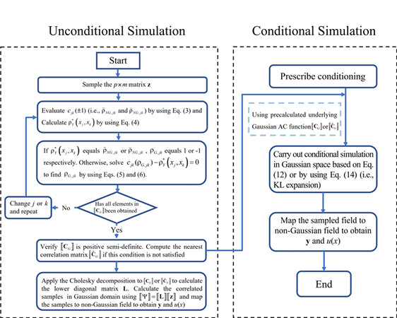
Figure 1. Flowchart of the proposed simulation procedure: the left panel represents the unconditional simulation, and the right panel shows the steps for the conditional simulation of the field.

2.2. Sampling of the simulated field by using the KL expansion

In the previous section, it is considered that the marginal CDF and the correlation function are prescribed for the nonhomogeneous non-Gaussian field. Moreover, $$ \left[\kern-0.15em\left[ {C_{\rho Y}} \right]\kern-0.15em\right]$$ (or $$ \left[\kern-0.15em\left[ {\tilde{C}_{\rho Y} ^\ast} \right]\kern-0.15em\right] $$ ) for the field at selected discrete points $$ [x]_p $$ is established, and the underlying Gaussian correlation matrix $$ \left[\kern-0.15em\left[ {C_{G}} \right]\kern-0.15em\right] $$ (or its corresponding nearest correlation matrix $$ \left[\kern-0.15em\left[ {\tilde{C}_{G}} \right]\kern-0.15em\right] $$ ) is obtained at $$ [x]_p $$ . For simplicity and without loss of generality, unless otherwise indicated, the notations $$ \left[\kern-0.15em\left[ {C_{G}} \right]\kern-0.15em\right] $$ and $$ \left[\kern-0.15em\left[ {C_{\rho Y}} \right]\kern-0.15em\right]$$ are replaced by $$ \left[\kern-0.15em\left[ {\tilde{C}_{G}} \right]\kern-0.15em\right] $$ and $$ \left[\kern-0.15em\left[ {\tilde{C}_{\rho Y} ^\ast} \right]\kern-0.15em\right] $$ in the following.

The use of $$ \left[\kern-0.15em\left[ {\tilde{C}_{\rho Y} ^\ast} \right]\kern-0.15em\right] $$ and KL expansion to simulate the non-Gaussian field by using an iterative procedure was presented in several studies[32, 33]. Since $$ \left[\kern-0.15em\left[ {\tilde{C}_{G}} \right]\kern-0.15em\right] $$ is already available, it can be used with the KL expansion to simulate the Gaussian field and map the simulated field to the non-Gaussian field through probability distribution transformation[35]. The application of the KL expansion has been considered in the literature[41].

For completeness and in order to provide the background for the conditional simulation based on the KL expansion, the use of the KL expansion is summarized below. In general, the random field (Gaussian or non-Gaussian) $$ Y(x) $$ can be expressed in the KL expansion[19, 32],

$$ \begin{equation} y(x)=\sum\limits_{q=1}^{\infty}{\sqrt{\lambda_q}f_q(x)w_q}, \end{equation} $$

where $$ w_q $$ represents independent zero-mean and unit variance random variables. For practical applications, the eigenvalue $$ \lambda_q $$ , and the eigenfunction $$ f_q(x_{,j}) $$ can be determined by solving Fredholm integral equation of the second kind[42] over the domain of the field $$ \omega $$ ,

$$ \begin{equation} \int_{\mathrm{\Omega}}{\rho(x_j,x_k)}f_q(x_j)dx_j=\lambda_qf_q(x_k), \end{equation} $$

By considering that the series shown in Equation (7) is truncated to the first few terms, an approximation to $$ y(x) $$ is obtained.

By taking advantage of the availability of $$ \left[\kern-0.15em\left[ {\tilde{C}_{G}} \right]\kern-0.15em\right] $$ , the practical implementation of simulating the Gaussian implementation by using the KL expansion can be written as[43],

$$ \begin{equation} [\psi]_{p}=\sum\limits_{q=1}^{p} \sqrt{\lambda_{q}}[\theta]_{p, q} w_{q}, \end{equation} $$

where $$ [\psi]_p $$ represents a sample of the Gaussian field at $$ [x]_p $$ with unit variance and correlation coefficient $$ \left[\kern-0.15em\left[ {\tilde{C}_{G}} \right]\kern-0.15em\right] $$ , the eigenvalue $$ \lambda_q $$ and eigenvector $$ [\theta]_{p,q} $$ are obtained by using the eigendecomposition or Cholesky decomposition and singular value decomposition to $$ \left[\kern-0.15em\left[ {\tilde{C}_{G}} \right]\kern-0.15em\right] $$ . For efficiency, Equation (9) can be truncated to the first $$ N $$ terms with $$ N \ll p $$ by retaining the first $$ N $$ terms with significant eigenvalues resulting in,

$$ \begin{equation} [\psi]_{p} \approx \sum\limits_{q=1}^{N} \sqrt{\lambda_{q}}[\theta]_{p, q} W_{q}, \end{equation} $$

By applying $$ F_{Y(x_j);x_j}^{-1}(\mathrm{\Phi}(\psi_j)) $$ , a sample of the non-Gaussian random field $$ [y]_p $$ is obtained, where $$ \psi_j j = 1,\cdots, p $$ , denotes the $$ j $$ -th element of $$ [\psi]_p $$ . Note that the type of approximation given in Equation (9) forms the basis for sparse sampling or compressive sensing[44].

2.3. Conditional simulation

Consider that the field to be simulated $$ Y(x) [i.e., U(x)] $$ is constrained by the observed values $$ y(x) $$ at $$ x=x_k $$ where $$ k $$ takes the index in $$ \mathrm{\Omega}_c=[k_1,k_2,\cdots,k_{nc}] $$ . To carry out the conditional simulation of the field $$ y(x) $$ at $$ x_j $$ for $$ j = 1,\cdots,p $$ but $$ j\notin\mathrm{\Omega}_c $$ , we note that the underlying Gaussian correlation matrix $$ \left[\kern-0.15em\left[ {\tilde{C}_{G}} \right]\kern-0.15em\right] $$ the field at $$ [x]_p $$ can be obtained based on the procedure shown in the flowchart depicted in Figure 1. Therefore, we could take advantage of the availability of $$ \left[\kern-0.15em\left[ {\tilde{C}_{G}} \right]\kern-0.15em\right] $$ to carry out conditional simulation for the nonhomogeneous non-Gaussian field. This could be done by first mapping the conditioning $$ y(x_k) $$ , for $$ k\in\mathrm{\Omega}_c $$ , to the Gaussian space using,

$$ \begin{equation} \psi(x)=\mathrm{\Phi}\left(F_{y(x);x}\left(y(x);x\right)\right),\ {\rm{ for }}\ x=x_k\ {\rm{ and }}\ k\in\mathrm{\Omega}_c, \end{equation} $$

Let $$ [\psi_\alpha] $$ denote the vector of size $$ nc\times 1 $$ for all the mapped conditioning in the Gaussian field. Similarly, let $$ [\psi_\beta] $$ denote the vector of size $$ (p-nc)\times 1 $$ containing the values of the (zero-mean and unit variance) Gaussian field for the remaining positions in the field $$ x_j $$ for $$ j $$ within $$ 1 $$ to $$ p $$ but $$ j\notin\mathrm{\Omega}_c $$ . The unknown values of the vector $$ [\psi_\beta] $$ conditioned on $$ [\psi_\alpha] $$ are governed by the following joint Gaussian distribution[37],

$$ \begin{equation} N\left(\left[\mu_{\beta \mid \alpha}\right]=\left[\kern-0.15em\left[ {C_{\beta \alpha}} \right]\kern-0.15em\right] \left[\kern-0.15em\left[ {C_{\alpha \alpha}^{-1}} \right]\kern-0.15em\right]\left[\psi_{\alpha}\right], \left[\kern-0.15em\left[ {\Sigma_{\beta \mid \alpha}} \right]\kern-0.15em\right]=\left[\kern-0.15em\left[ {C_{\beta \beta}} \right]\kern-0.15em\right]-\left[\kern-0.15em\left[ {C_{\beta \alpha}} \right]\kern-0.15em\right] \left[\kern-0.15em\left[ {C_{\alpha \alpha}^{-1}} \right]\kern-0.15em\right] \left[\kern-0.15em\left[ {C_{\alpha \beta}} \right]\kern-0.15em\right]\right) \end{equation} $$

where $$ N(\ ,\ ) $$ denotes the multi-dimensional normal distribution with $$ [\mu_{\beta \mid \alpha}] $$ and $$ \left[\kern-0.15em\left[ {\Sigma_{\beta \mid \alpha}} \right]\kern-0.15em\right] $$ represent the mean vector and covariance matrix, and C with subscript denotes submatrices that form the correlation coefficient matrix of the vector of $$ [[\psi_{\alpha}]^{T},[\psi_{\beta}]^{T}]^{T} $$ ,

$$ \left[\!\left[ \begin{array}{*{35}{l}} {{C}_{\alpha \alpha }} & {{C}_{\alpha \beta }} \\ {{C}_{\beta \alpha }} & {{C}_{\beta \beta }} \\ \end{array} \right]\!\right] $$

This matrix can be constructed by rearranging $$ \left[\kern-0.15em\left[ {\tilde{C}_{G}} \right]\kern-0.15em\right] $$ of the field represented at discretized points of the field at $$ j = 1, \cdots, p. $$

By generating $$ m $$ conditional samples of $$ [\psi_\beta] $$ based on Equation (12) [see also Equation (1)], transforming each sampled value to $$ y(x) $$ by using $$ F_{Y(x);x}^{-1}(\mathrm{\Phi}(\psi)) $$ , and calculating $$ u(x)=\mu_{U(x)}+\sigma_{U(x)}y(x) $$ , samples of the non-Gaussian fields are obtained, which complements the conditioning value to describe the conditional random field. This conditional simulation algorithm for the nonhomogeneous non-Gaussian field is very simple to use [Figure 1] as the conditional Gaussian simulation by using Equation (12) is straightforward.

We also note that a method[34] was developed to carry out the conditional simulation of the Gaussian field based on the KL expansion. It can be shown that their method for the underlying Gaussian random field at $$ p $$ discretized points $$ [x]_p, [\tilde{\psi}]_p $$ , [i.e., analog to Equation (7) vs. Equation (9)] for the given $$ \left[\kern-0.15em\left[ {\tilde{C}_{G}} \right]\kern-0.15em\right] $$ can be written as,

$$ \begin{equation} [\tilde{\psi}]_{p}=\sum\limits_{q=1}^{p} \sqrt{\eta_{q}}[h]_{p, q}\left(\tilde{\mu}_{q}+\sum\limits_{j=1}^{p} \tilde{S}_{q, j} u_{j}\right), \end{equation} $$

where the eigenvalue $$ \lambda_q $$ and eigenvector $$ [h]_{p,q} $$ are obtained by applying the eigendecomposition. In Equation (14), $$ {\tilde{\mu}}_q $$ denotes the $$ q $$ -th element of the conditional mean $$ [\tilde{\mu}]q $$ of the size $$ p\times 1 $$ that is given by,

$$ \begin{equation} [\tilde{\mu}]_{p}=\left[\kern-0.15em\left[ { \sqrt{\eta} } \right]\kern-0.15em\right] \left[\kern-0.15em\left[ { G } \right]\kern-0.15em\right]^{T}\left(\left[\kern-0.15em\left[ { G } \right]\kern-0.15em\right] \left[\kern-0.15em\left[ { \sqrt{\eta} } \right]\kern-0.15em\right]^{2} \left[\kern-0.15em\left[ { G } \right]\kern-0.15em\right]^{T}\right)^{-1}\left[\psi_{\alpha}\right], \end{equation} $$

and $$ {\tilde{S}}_{q,j} $$ denotes the $$ (q,j) $$ -the element of the matrix $$ \left[\kern-0.15em\left[ { \tilde{S} } \right]\kern-0.15em\right] $$ of the size $$ p\times p $$ that is given by,

$$ \begin{equation} \left[\kern-0.15em\left[ { \tilde{S} } \right]\kern-0.15em\right]=\left[\kern-0.15em\left[ { I } \right]\kern-0.15em\right]-\left[\kern-0.15em\left[ { \sqrt{\eta} } \right]\kern-0.15em\right] \left[\kern-0.15em\left[ { G } \right]\kern-0.15em\right]^{T}\left(\left[\kern-0.15em\left[ { G } \right]\kern-0.15em\right] \left[\kern-0.15em\left[ { \sqrt{\eta} } \right]\kern-0.15em\right]^{2} \left[\kern-0.15em\left[ { G } \right]\kern-0.15em\right]^{T}\right)^{-1} \left[\kern-0.15em\left[ { G } \right]\kern-0.15em\right] \left[\kern-0.15em\left[ { \sqrt{\eta} } \right]\kern-0.15em\right]. \end{equation} $$

where $$ \left[\kern-0.15em\left[ { I } \right]\kern-0.15em\right] $$ is the $$ p\times p $$ identity matrix, $$ \left[\kern-0.15em\left[ { G } \right]\kern-0.15em\right] $$ is an $$ nc\times p $$ submatrix of $$ \left[\kern-0.15em\left[ { h } \right]\kern-0.15em\right] $$ , in which the $$ j $$ -th column of $$ \left[\kern-0.15em\left[ { G } \right]\kern-0.15em\right] $$ is formed by the $$ k $$ -th elements of the $$ j $$ -th column of $$ \left[\kern-0.15em\left[ { h } \right]\kern-0.15em\right] $$ with the index $$ k\in\mathrm{\Omega}_c $$ .

Once $$ \tilde{\psi}(x) $$ or $$ [\tilde{\psi}]_p $$ is sampled, the conditional field $$ y(x) $$ or $$ [y]_p $$ is obtained by using $$ F_{Y(x_j);x_j}^{-1}(\mathrm{\Phi}({\tilde{\psi}}_j)) $$ . The flowchart for the conditional simulation is included in Figure 1, whether the conditional Gaussian model shown in Equation (12) or by using the KL expansion model shown in Equation (14) is considered. The use of Equation (12) requires the simulation of the correlated Gaussian random variables, which can be done by applying the Cholesky decomposition [Equation (1)]. The use of Equation (14) requires the evaluation of eigenvalues and eigenvectors if they are unavailable. In both cases, the use of probability transformation is required, and the steps are straightforward, as shown in Figure 1.

2.4. Discussion on the extension to the multi-dimensional random field

In this section, we highlight steps to extend the procedure described in the previous section to the $$ n $$ -dimensional case. Consider the case of simulating the $$ n $$ -dimensional zero-mean and unit variance random field that is defined over the domain of x, with the value represented by $$ y $$ (x), where $$ x=[x_1,\cdots,x_n] $$ . The field is defined by the prescribed marginal CDF, $$ F_{y(x);x}(y(x);x) $$ , and the correlation coefficient function. Similar to the one-dimensional field case, it is considered that the field is to be simulated at a set of discrete points that are denoted as $$ x_N=[x_{1,j_1},\cdots,x_{n,j_n}] $$ , where $$ [j]=[j_1,\cdots,j_n] $$ , $$ j_k=1,\cdots,p_k, $$ $$ p_k $$ denotes the total number of points along the $$ x_k $$ -axis, and $$ N $$ represents the total number of points (i.e., combinations of $$ j_k,\; k = 1,\cdots, n $$ , which equals $$ \prod_{k=1}^{n}p_k) $$ within the $$ n $$ -dimensional field to be considered. The correlation coefficient matrix for the random field represented at the discretized points is to be calculated based on the prescribed correlation coefficient function. In other words, we treat a multi-dimensional field by vectorizing it into a long one-dimensional vector, and the procedure described in the previous sections can be directly applied. Perhaps, the manipulation of the $$ n $$ indices in [j] for the points in the $$ n $$ -dimensional space could be tedious. A systematic ordering of the index could facilitate the computer program task.

Since the extension to the multi-dimensional field is straightforward, no further consideration for the $$ n $$ -dimensional case is made.

3. ILLUSTRATIVE EXAMPLES

3.1. Examples of using the proposed procedure to evaluate underlying Gaussian correlation and unconditional simulation

Several numerical examples are presented by considering the homogeneous/nonhomogeneous processes with weakly and strongly non-Gaussian processes to illustrate the applicability of the proposed procedures depicted in Figure 1.

The examples in this subsection were considered in the literature[32, 35]. The assumed marginal distributions and the AC function for the homogeneous non-Gaussian cases (i.e., Cases 1 to 8) are listed in Table 1. The use of the beta distribution described in the table leads to a weakly non-Gaussian field, while the use of the lognormal distribution described in the table results in a strongly non-Gaussian field.

Table 1

Definition of the cases (see [35])

CasePrescribed autocorrelation function for homogeneous and nonhomogeneous cases Cases 1 to 4 are homogeneous Cases 4 to 8 are nonhomogeneousDistribution type and notes
Beta distributionLognormal distribution
1$$ C_{\rho 1}\left(x_{j}, x_{k}\right)=\exp \left(-\left|x_{j}-x_{k}\right|\right)$$ $$ \begin{aligned} &F(y)=\frac{\Gamma(p) \Gamma(q)}{\Gamma(p+q)} \int_{0}^{u} z^{p-1}(1-z)^{q-1} d z \\ &p=4, q=2 \text {. } \\ &\text {For the Cases } 1 \text { to } 4 \text {, } \\ &u=(y+3.74) /(1.87+3.74) \text {. } \\ &\text {The field is defined for } x \text { within } 0 \\ &\text {to } 2 \text { and discretized using } \Delta x=0.02 \text {. } \\ &\text {For the Cases } 5 \text { to } 8 \text {, } \\ &u=\left(y-y_{\min }\right) /\left(y_{\max }-y_{\min }\right), \\ &y_{\min }=\mu_{b}\left(x_{j}\right)-\sigma_{b}\left(x_{j}\right) \sqrt{\frac{p(p+q+1)}{q}}, \\ &y_{\max }=\mu_{b}\left(x_{j}\right)+\sigma_{b}\left(x_{j}\right) \sqrt{\frac{q(p+q+1)}{p}}. \\ &\text {The mean } \mu_{b}\left(x_{j}\right)=0 \text { and the standard } \\ &\text {deviation } \sigma_{b}\left(x_{j}\right) \text { could be obtained based } \\ &\text {on the autocovariance function. The field is } \\ &\text {defined for } x \text { within } 0 \text { to } 1 \text { and discretized } \\ &\text {using } \Delta x=0.01 . \end{aligned}$$ $$ \begin{aligned} &F(y)=F\left(\frac{\ln (y-\delta)-\alpha}{\beta}\right),\\ &\beta=1 \text {. }\\ &\text {For the Cases 1 to 4} ,\\ &\alpha=-0.7707\ \text {and}\ \delta=-0.7628.\\ &\text {The field is defined for}\ x\ \text {within 0 to 2 and}\\ &\text {discretized using}\ \Delta x=0.02.\\ &\text {For the Cases 5 to 8}, \alpha\left(x_{j}\right)\text { and }\delta\left(x_{j}\right)\\ &\text {could be obtained by solving the equations}\\ &\text {below},\\ &\mu_{l}\left(x_{j}\right)=\delta\left(x_{j}\right)+\exp \left[\alpha\left(x_{j}\right)+\frac{\beta^{2}}{2}\right], \\ &\sigma_{l}^{2}\left(x_{j}\right)=\left[\exp \left(\beta^{2}\right)-1\right]\\ &\ \ \ \ \ \ \ \ \ \ \times \exp \left[2 \alpha\left(x_{j}\right)+\beta^{2}\right] .\\ &\text {The mean }\mu_{l}\left(x_{j}\right)=0\text { and the variance }\\ &\sigma_{l}^{2}\left(x_{j}\right)\text { could be obtained based on the }\\ &\text {autocovariance function. The field is }\\ &\text {defined for }x\text { within 0 to 1 and }\\ &\text {discretized using }\Delta x=0.01. \end{aligned}$$
2$$ C_{\rho 2}\left(x_{j}, x_{k}\right)=\exp \left(-\left|x_{j}-x_{k}\right|^{2}\right)$$
3$$ \begin{aligned} C_{\rho 3}\left(x_{j}, x_{k}\right)&=\exp \left(-\left|x_{j}-x_{k}\right|\right)\\ &\times \cos \left(4 \pi\left(x_{j}-x_{k}\right)\right) \end{aligned}$$
4$$ \begin{aligned} C_{\rho 4}\left(x_{j}, x_{k}\right)&=\exp \left(-\left|x_{j}-x_{k}\right|^{2}\right)\\ &\times \cos \left(4 \pi\left(x_{j}-x_{k}\right)\right) \end{aligned}$$
5$$C_{\rho 5}\left(x_{j}, x_{k}\right)=\min \left(x_{j}, x_{k}\right)$$
6$$ \begin{aligned} C_{\rho 6}\left(x_{j}, x_{k}\right)&=4\left(\min \left(x_{j}, x_{k}\right)\right.\\ &\left.-x_{j} x_{k}\right) \end{aligned}$$
7$$ \begin{aligned} C_{\rho 7}\left(x_{j}, x_{k}\right)&=\min \left(x_{j}, x_{k}\right)\\ &\times \cos \left(4 \pi\left(x_{j}-x_{k}\right)\right) \end{aligned}$$
8$$ C_{\rho 8}\left(x_{j}, x_{k}\right)$$

First, for each of the considered homogeneous cases, the application of the proposed procedure shown in Figure 1 is employed. For the analysis, samples of the independent standard normally distributed random variables are simulated for a sample size $$ m = 50,000 $$ . This sample size is used throughout the numerical analysis in the present study. The selection of $$ m = 50,000 $$ is based on a sensitivity analysis, indicating that the use of $$ m = 10,000 $$ to $$ 100,000 $$ is adequate for most considered cases. An increased $$ m $$ results in an increased computing time. The selection is also based on balancing the accuracy and computing time. These samples are used to evaluate the bounds $$ \hat{\rho}_{N G, j k} $$ and $$ {\breve{\rho}}_{NG,jk} $$ . Based on the bounds shown in Equations (3) and (4), $$ \left[\kern-0.15em\left[ {C_{\rho Y} ^\ast} \right]\kern-0.15em\right] $$ is obtained, and the corresponding underlying Gaussian matrix $$ \left[\kern-0.15em\left[ {C_{G}} \right]\kern-0.15em\right] $$ is determined by using the bisection method and verified using the optimization approach formulated in Equation (6). In all cases, the obtained $$ \rho_{G,jk} $$ values by both approaches are practically identical. Since the same conclusion is observed for the remaining numerical examples, only the bisection method is used to calculate $$ \rho_{G,jk} $$ for the remaining numerical examples. Note that the use of the bisection method leads to an error (i.e., the last bracketed interval) of less than approximately $$ 1/2^{n_I} $$ , where $$ n_I $$ is the number of iterations. Therefore, an iteration of 7, 10, 13, and 17 leads to the absolute value of the error less than about $$ 1 \times 10^{-2} $$ , $$ 1 \times 10^{-3} $$ , $$ 1 \times 10^{-4} $$ , and $$ 1 \times 10^{-5} $$ . $$ n_I $$ less than 16 is used for all the computations. Moreover, a verification that $$ \left[\kern-0.15em\left[ {C_{G}} \right]\kern-0.15em\right] $$ is positive semi-definite is carried out. $$ \left[\kern-0.15em\left[ {C_{G}} \right]\kern-0.15em\right] $$ is replaced by its corresponding nearest correlation matrix[18]$$ \left[\kern-0.15em\left[ {\tilde{C}_{G}} \right]\kern-0.15em\right] $$ if such a condition is not satisfied. Finally, the non-Gaussian field is simulated following the steps shown in Figure 1, and the AC function of simulated samples is calculated. The target AC function and the AC functions based on $$ \left[\kern-0.15em\left[ {C_{\rho Y} ^\ast} \right]\kern-0.15em\right] $$ and $$ \left[\kern-0.15em\left[ {C_{G}} \right]\kern-0.15em\right] $$ are presented in Figure 2 and Figure 3. For cases, when $$ \left[\kern-0.15em\left[ {\tilde{C}_{G}} \right]\kern-0.15em\right] $$ and $$ \left[\kern-0.15em\left[ {\tilde{C}_{\rho Y} ^\ast} \right]\kern-0.15em\right] $$ are calculated, they are shown in Figure 2 and Figure 3.

Unconditional and conditional simulation of nonstationary and non-Gaussian vector and field with prescribed marginal and correlation by using iteratively matched correlation

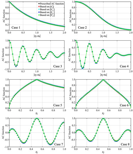
Figure 2. Comparison of the prescribed AC function, estimated AC function based on samples, and underlying Gaussian AC function for Cases 1 to 8 by considering that the marginal distribution is the beta distribution shown in Table 1. The plots for Cases 5 to 8, considered $$ x_k = 0.5 $$ . AC: Autocorrelation.

Unconditional and conditional simulation of nonstationary and non-Gaussian vector and field with prescribed marginal and correlation by using iteratively matched correlation

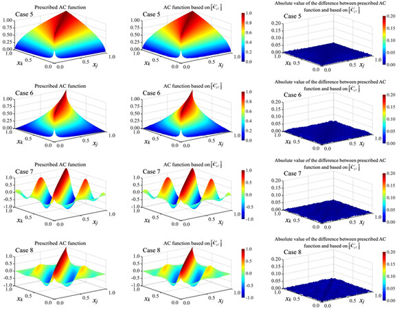
Figure 3. Comparison of the prescribed AC function, estimated AC function based on samples, and their differences for Cases 5 to 8. The considered marginal distribution is the beta distribution shown in Table 1. AC: Autocorrelation.

The results presented in Figure 2 and Figure 3 indicate that the underlying Gaussian AC functions are close to the target AC functions. The closeness is because the use of the beta distribution presented in Table 1 as the marginal distribution leads to only weakly non-Gaussian fields for the considered cases. The weakly non-Gaussian behavior was noted in the literature[35]. For Cases 2 and 4 (for the considered grid system), it is observed that $$ \left[\kern-0.15em\left[ {C_{G}} \right]\kern-0.15em\right] $$ cannot be decomposed by the Cholesky decomposition. Therefore, its nearest correlation matrix $$ \left[\kern-0.15em\left[ {\tilde{C}_{G}} \right]\kern-0.15em\right] $$ is calculated and used as the basis to simulate the non-Gaussian field. The corresponding $$ \left[\kern-0.15em\left[ {\tilde{C}_{\rho Y} ^\ast} \right]\kern-0.15em\right] $$ is calculated from the simulated non-Gaussian field. The plots shown in Figure 2 indicate that the differences between $$ \left[\kern-0.15em\left[ {C_{G}} \right]\kern-0.15em\right] $$ and $$ \left[\kern-0.15em\left[ {\tilde{C}_{G}} \right]\kern-0.15em\right] $$ and between $$ \left[\kern-0.15em\left[ {C_{\rho Y}} \right]\kern-0.15em\right]$$ and $$ \left[\kern-0.15em\left[ {\tilde{C}_{\rho Y} ^\ast} \right]\kern-0.15em\right] $$ are very small. A further inspection of the numerical results indicates that the absolute value of the difference between the elements in $$ \left[\kern-0.15em\left[ {C_{G}} \right]\kern-0.15em\right] $$ and its corresponding element in $$ \left[\kern-0.15em\left[ {\tilde{C}_{G}} \right]\kern-0.15em\right] $$ is much less than 0.01.

The plots for Cases 5 to 8 shown in Figure 2 are those calculated for $$ x_j = 0.5 $$ and by varying $$ x_k $$ within 0 to 1. Since Cases 5 to 8 are nonhomogeneous, the surfaces for their prescribed AC functions and for $$ \left[\kern-0.15em\left[ {\tilde{C}_{\rho Y} ^\ast} \right]\kern-0.15em\right] $$ are presented in Figure 3, indicating that the latter mimics the former well. In addition, a quantitative comparison of the difference between the prescribed AC function and that based on $$ \left[\kern-0.15em\left[ {\tilde{C}_{\rho Y} ^\ast} \right]\kern-0.15em\right] $$ is presented in Figure 3. The differences are caused by the use of the limited samples (i.e., a sample size of 50000) as well as the use of the nearest correlation matrix. In all cases, the small differences presented in the figure confirm the adequacy of the procedure depicted in Figure 1.

By repeating the analysis that is carried out for the results presented in Figure 2 and Figure 3 but replacing the beta distribution with the lognormal distribution shown in Table 1, the obtained results are shown in Figure 4 and Figure 5. As pointed out in the study[35], the use of this lognormal distribution results strongly non-Gaussian field. This strongly non-Gaussian behavior is reflected in the calculated underlying Gaussian AC functions.

Unconditional and conditional simulation of nonstationary and non-Gaussian vector and field with prescribed marginal and correlation by using iteratively matched correlation

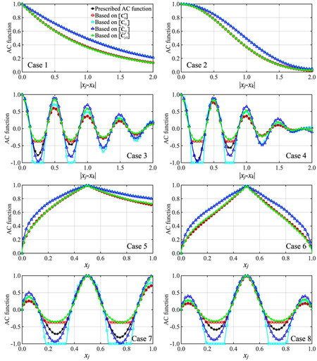
Figure 4. Comparison of the prescribed AC function, estimated AC function based on samples, and underlying Gaussian AC function for Cases 1 to 8 by considering that the marginal distribution is the lognormal distribution shown in Table 1. The plots for Cases 5 to 8, considered $$ x_k = 0.5 $$ . AC: Autocorrelation.

Unconditional and conditional simulation of nonstationary and non-Gaussian vector and field with prescribed marginal and correlation by using iteratively matched correlation

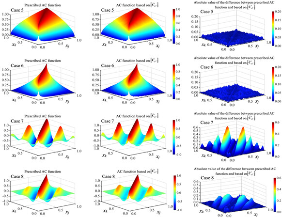
Figure 5. Comparison of the prescribed AC function, estimated AC function based on samples, and their differences for Cases 5 to 8. The considered marginal distribution is the lognormal distribution shown in Table 1. AC: Autocorrelation.

The plots presented in Figure 4 for Cases 3, 4, 7, and 8 indicate that there are segments where $$ \rho_{G,jk} $$ equals $$ -1 $$ . This is because the calculated $$ \rho_Y(x_j,x_k) $$ is less than $$ {\breve{\rho}}_{NG,jk} $$ [see Equation (4)]. For these cases, $$ \left[\kern-0.15em\left[ {C_{\rho Y} ^\ast} \right]\kern-0.15em\right] $$ and $$ \left[\kern-0.15em\left[ {C_{G}} \right]\kern-0.15em\right] $$ are calculated. Since an assessment indicates that $$ \left[\kern-0.15em\left[ {C_{G}} \right]\kern-0.15em\right] $$ does not form a proper correlation coefficient matrix, its corresponding nearest correlation matrix $$ \left[\kern-0.15em\left[ {\tilde{C}_{G}} \right]\kern-0.15em\right] $$ is then calculated by using the algorithm given in the study[18]. The non-Gaussian field is then simulated based on $$ \left[\kern-0.15em\left[ {\tilde{C}_{G}} \right]\kern-0.15em\right] $$ using the procedure described in Figure 1 and $$ \left[\kern-0.15em\left[ {\tilde{C}_{\rho Y} ^\ast} \right]\kern-0.15em\right] $$ is evaluated based on the simulated fields.

The plots presented in Figure 4 for Cases 3, 4, 7, and 8 show that $$ \left[\kern-0.15em\left[ {\tilde{C}_{\rho Y} ^\ast} \right]\kern-0.15em\right] $$ can deviate from their target. The differences illustrate the well-known limitation of using the Nataf translation system to represent the non-Gaussian field[12-14, 16, 35] rather than the numerical procedure used in the present study.

Figure 5 shows the surface of the target AC functions and the surface of the underlying Gaussian AC functions. In the same figure, the differences between the surface of the target AC function and the surface of $$ \left[\kern-0.15em\left[ {\tilde{C}_{\rho Y} ^\ast} \right]\kern-0.15em\right] $$ are also depicted. The large differences between the prescribed AC function and that based on $$ \left[\kern-0.15em\left[ {\tilde{C}_{\rho Y} ^\ast} \right]\kern-0.15em\right] $$ for some regions of the field can be explained based on the arguments used to explain the results presented in Figure 4.

3.2. Examples using the KL expansion to simulate non-Gaussian field

In this subsection, we consider again all cases shown in Table 1 but use the KL expansion to augment the simulated field. For the analysis, we take advantage of the availability of $$ \left[\kern-0.15em\left[ {C_{G}} \right]\kern-0.15em\right] $$ and $$ \left[\kern-0.15em\left[ {C_{\rho Y}} \right]\kern-0.15em\right]$$ (if they are not proper correlation matrices, we use their corresponding nearest correlation matrices $$ \left[\kern-0.15em\left[ {\tilde{C}_{G}} \right]\kern-0.15em\right] $$ and $$ \left[\kern-0.15em\left[ {\tilde{C}_{\rho Y} ^\ast} \right]\kern-0.15em\right] $$ ), that is discussed in the previous section.

First, the eigendecomposition is applied to
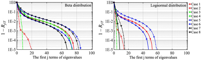
 $$ \left[\kern-0.15em\left[ {\tilde{C}_{G}} \right]\kern-0.15em\right] $$ (or $$ \left[\kern-0.15em\left[ {C_{G}} \right]\kern-0.15em\right] $$ if it is a proper correlation matrix) for each of Cases 1 to 8. By sorting the eigenvalues in descending order, we sum up the eigenvalues of the first $$ j $$ terms and normalize them with respect to the sum of all the eigenvalues. The normalized value, denoted as $$ R_{j/T} $$ is plotted in Figure 6 for each case, indicating that $$ R_{j/T} $$ is greater than about 0.95. This indicates that the consideration of the first 21 terms of the KL expansion [see Equation (10)] could provide adequate representations of the considered random fields.

Unconditional and conditional simulation of nonstationary and non-Gaussian vector and field with prescribed marginal and correlation by using iteratively matched correlation

Figure 6. Value of $$ R_{j/T} $$ for the considered cases showing the contribution of the eigenvalues from the first $$ j $$ terms.

We use the obtained $$ \left[\kern-0.15em\left[ {\tilde{C}_{G}} \right]\kern-0.15em\right] $$ , considering $$ N = 21 $$ , applying Equation (10) and employing the probability transformation mapping to simulate the non-Gaussian random field at points with the separation between two adjacent points $$ \delta x = 0.1 $$ for Cases 1 to 4, and with $$ \delta x = 0.05 $$ for Cases 5 to 8. An illustration of five samples for each case is depicted in Figure 7. By generating 50, 000 samples for each case, the calculated correlation coefficient is presented in Figure 8 and compared with $$ \left[\kern-0.15em\left[ {\tilde{C}_{\rho Y} ^\ast} \right]\kern-0.15em\right] $$ that is obtained in the previous section (i.e., based on the procedure shown on the left panel in Figure 1). The comparison indicates that the correlation obtained from the samples agrees well with $$ \left[\kern-0.15em\left[ {\tilde{C}_{\rho Y} ^\ast} \right]\kern-0.15em\right] $$ .

Unconditional and conditional simulation of nonstationary and non-Gaussian vector and field with prescribed marginal and correlation by using iteratively matched correlation

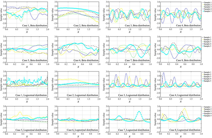
Figure 7. Typical samples obtained by applying the KL expansions and probability transformation mapping for each of the cases listed in Table 1. The first two rows are obtained by considering the beta distribution presented in Table 1 and the last two rows are obtained by considering the lognormal distribution presented in Table 1. KL: Karhunen-Loeve.

Unconditional and conditional simulation of nonstationary and non-Gaussian vector and field with prescribed marginal and correlation by using iteratively matched correlation

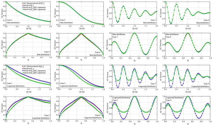
Figure 8. Comparison of the calculated correlation coefficient from the sampled random field to $$ \left[\kern-0.15em\left[ { \tilde{C}_{\rho Y}^{*} } \right]\kern-0.15em\right] $$ obtained from the sampled random field based on the proposed procedure depicted on the left panel shown in Figure 1. The first two rows are obtained by considering the beta distribution presented in Table 1 and the last two rows are obtained by considering the lognormal distribution presented in Table 1.

3.3. Examples of conditional simulation

For illustrating the conditional simulation, we consider Cases 1 and 5. By assuming that the marginal distribution is the beta or lognormal distribution shown in Table 1, we sample a field at $$ p = 101 $$ points for the considered case. We select 5 points from the sampled field as the conditioning points that are shown in Figure 9. We then apply the procedure described in Figure 1 to sample the random fields conditionally. Five samples for each considered case are presented in Figure 9 by using Equation (12). As shown in the figure, the sampled random fields are constrained by the conditioning points.

Unconditional and conditional simulation of nonstationary and non-Gaussian vector and field with prescribed marginal and correlation by using iteratively matched correlation

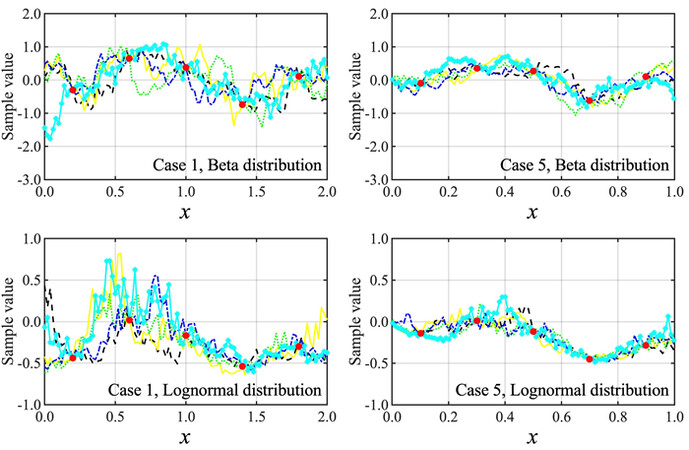
Figure 9. Five conditionally sampled fields for Cases 1 and 5. The large dots represent the conditioning points and the lines represent the sampled fields.

4. CONCLUSIONS

A sample-based numerical procedure to estimate the underlying Gaussian correlation for a homogeneous/nonhomogeneous non-Gaussian field is proposed in the present study. The estimation is based on the Nataf translation framework and takes advantage that the range of feasible correlation coefficients for non-Gaussian random variables by using the translation is bounded. Numerical examples show that the proposed estimation procedure is effective and can be used directly to identify whether the underlying Gaussian correlation that leads to exactly matching the prescribed correlation can be found. It is shown that by taking into account the bounds, the underlying Gaussian correlation can be easily found by using the simple bisection method or optimization algorithm. From the numerical example, it was noted that $$ \left[\kern-0.15em\left[ {C_{G}} \right]\kern-0.15em\right] $$ may not be a positive semi-definite matrix (as noted by other researchers). In such a case, its corresponding nearest correlation matrix $$ \left[\kern-0.15em\left[ {\tilde{C}_{G}} \right]\kern-0.15em\right] $$ is used; a detailed inspection of the numerical results indicates that the absolute value of the differences between the elements in $$ \left[\kern-0.15em\left[ {C_{G}} \right]\kern-0.15em\right] $$ and its corresponding element in $$ \left[\kern-0.15em\left[ {\tilde{C}_{G}} \right]\kern-0.15em\right] $$ is much less than 0.01.

We also present the steps to augment the simulated non-Gaussian field for a refined discretized grid of the random field by applying the KL expansion and using samples obtained for a much more coarse grid system. The procedure is illustrated through numerical examples.

It was shown that the conditional simulation could easily be carried out within the established simulation framework, and the extension of the procedure to the multi-dimensional random field case is straightforward.

DECLARATIONS

Acknowledgments

We gratefully acknowledge the financial support received from the Natural Sciences and Engineering Research Council of Canada (RGPIN-2016-04814, for HPH), the China Scholarship Council (No. 201807980004 for MYX), and the University of Western Ontario.

Authors' contributions

Investigation, Methodology, Formal analysis, Writing - original draft, Writing - review & editing: Xiao MY

Conceptualization, Funding acquisition, Investigation, Methodology, Project administration, Resources, Supervision, Writing - original draft, Writing - review & editing: Hong H

Availability of data and materials

Some or all data, models, or code generated or used during the study are available from the author by request.

Financial support and sponsorship

The authors acknowledge the financial support received from the Natural Sciences and Engineering Research Council of Canada (RGPIN-2016-04814, for HPH) and the China Scholarship Council (No.201807980004, for MYX).

Conflicts of interest

All authors declared that there are no conflicts of interest.

Ethical approval and consent to participate

Not applicable.

Consent for publication

Not applicable.

Copyright

© The Author(s) 2022.

REFERENCES

1. Ang AHS, Tang WH. Probability concepts in engineering planning and design, vol. 2: Decision, risk, and reliability. New York, NY, USA: John Wiley & Sons, Inc.; 1984.

2. Madsen HO, Krenk S, Lind NC. Methods of structural safety Mineola, New York: Dover Publications, Inc.; 2006.

3. Melchers RE, Beck AT. Structural reliability analysis and prediction. New York, NY, USA: John Wiley & Sons, Inc.; 2018. Available from: https://www.wiley.com/en-hk/Structural+Reliability+Analysis+and+Prediction%2C+3rd+Edition-p-9781119265993 [Last accessed on 9 May 2022].

4. Nataf A. Determination des distribution don t les marges sont donnees. Comptes Rendus Acad Sci 1962;225:42-3.

5. Grigoriu M. Simulation of stationary Non-Gaussian translation processes. J Eng Mech 1998;124:121-6.

6. Chen H. Initialization for NORTA: Generation of random vectors with specified marginals and correlations. INFORMS J Comput 2001;13:312-31.

7. Embrechts P, McNeil AJ, Straumann D. Correlation and dependence in risk management: properties and pitfalls. In: Dempster MAH, editor. Risk management: value at risk and beyond. Cambridge: Cambridge University Press; 2002. pp. 176-223.

8. Fleishman AI. A method for simulating non-normal distributions. Psychometrika 1978;43:521-32.

9. Winerstein SR. Nonlinear vibration models for extremes and fatigue. J Eng Mech 1988;114:1772-90.

10. Zhao Y, Zhang X, Lu Z. A flexible distribution and its application in reliability engineering. Reliab Eng Syst Saf 2018;176:1-12.

11. Lu Z, Zhao Z, Zhang X, Li C, Ji X, Zhao Y. Simulating stationary non-gaussian processes based on unified hermite polynomial model. J Eng Mech 2020;146:04020067.

12. Li ST, Hammond JL. Generation of pseudorandom numbers with specified univariate distributions and correlation coefficients. IEEE Trans Syst Man Cybern 1975;SMC-5:557-61.

13. Liu P, Der Kiureghian A. Multivariate distribution models with prescribed marginals and covariances. Probabilist Eng Mech 1986;1:105-12.

14. Lurie PM, Goldberg MS. An approximate method for sampling correlated random variables from partially-specified distributions. Manag Sci 1998;44:203-18.

15. Yang I. Distribution-free Monte Carlo simulation: premise and refinement. J Constr Eng Manag 2008;134:352-60.

16. Cario MC, Nelson BL. Modeling and generating random vectors with arbitrary marginal distributions and correlation matrix, technical report. Evanston, IL: Department of Industrial Engineering and Management Sciences, Northwestern University; 1997. [Last accessed on 9 May 2022].

17. Higham NJ. Computing the nearest correlation matrix - a problem from finance. IMA J Numer Anal 2002;22:329-43.

18. Qi H, Sun D. A quadratically convergent newton method for computing the nearest correlation matrix. SIAM J Matrix Anal Appl 2006;28:360-85.

19. Ghanem RG, Spanos PD. Stochastic finite elements: a spectral approach. Mineola, NY, USA: Courier Corporation; 2003. Available from: https://link.springer.com/book/10.1007/978-1-4612-3094-6 [Last accessed on 9 May 2022].

20. Shinozuka M, Jan C. Digital simulation of random processes and its applications. J Sound Vib 1972;25:111-28.

21. Yang J. Simulation of random envelope processes. J Sound Vib 1972;21:73-85.

22. Shinozuka M, Deodatis G. Simulation of multi-dimensional gaussian stochastic fields by spectral representation. Appl Mech Rev 1996;49:29-53.

23. Yamazaki F, Shinozuka M. Digital generation of non-Gaussian stochastic fields. J Eng Mech 1988;114:1183-97.

24. Deodatis G, Micaletti RC. Simulation of highly skewed non-Gaussian stochastic processes. J Eng Mech 2001;127:1284-95.

25. Ferrante F, Arwade S, Graham-brady L. A translation model for non-stationary, non-Gaussian random processes. Probabilist Eng Mech 2005;20:215-28.

26. Shields M, Deodatis G. Estimation of evolutionary spectra for simulation of non-stationary and non-Gaussian stochastic processes. Comput Struct 2013;126:149-63.

27. Vanmarcke EH, Fenton GA. Conditioned simulation of local fields of earthquake ground motion. Struct Saf 1991;10:247-64.

28. Kameda H, Morikawa H. Conditioned Stochastic processes for conditional random fields. J Eng Mech 1994;120:855-75.

29. Hu L, Xu YL, Zheng Y. Conditional simulation of spatially variable seismic ground motions based on evolutionary spectra. Earthq Eng Struct Dyn 2012;41:2125-39.

30. Cui XZ, Hong HP. Conditional simulation of spatially varying multicomponent nonstationary ground motions: bias and Ill condition. J Eng Mech 2020;146:04019129.

31. Zhang J, Ellingwood B. Orthogonal series expansions of random fields in reliability analysis. J Eng Mech 1994;120:2660-77.

32. Phoon K, Huang S, Quek S. Simulation of second-order processes using Karhunen-Loeve expansion. Comput Struct 2002;80:1049-60.

33. Phoon K, Huang H, Quek S. Simulation of strongly non-Gaussian processes using Karhunen-Loeve expansion. Probabilist Eng Mech 2005;20:188-98.

34. Ossiander ME, Peszynska M, Vasylkivska VS. Conditional stochastic simulations of flow and transport with karhunen-loève expansions, stochastic collocation, and sequential gaussian simulation. J Appl Math 2014;2014:1-21.

35. Kim H, Shields MD. Modeling strongly non-Gaussian non-stationary stochastic processes using the iterative translation approximation method and Karhunen-Loève expansion. Comput Struct 2015;161:31-42.

36. Zheng Z, Dai H. Simulation of multi-dimensional random fields by Karhunen-Loève expansion. Comput Methods Appl Mech Eng 2017;324:221-47.

37. Anderson TW. An introduction to multivariate statistical analysis (Vol. 2). New York, NY, USA: Wiley; 2003. pp. 5-13.

38. Stuart A, Arnold S, Ord JK, O'Hagan A, Forster J. Kendall's advanced theory of statistics New York, NY, USA: Wiley. Inc.; 1994.

39. Tong YL. The Multivariate normal distribution. New York, NY, USA: Springer; 1990. pp. 181-201.

40. Higham NJ. Analysis of the cholesky decomposition of a semi-definite matrix. Oxford University Press; 1990. Available from: http://eprints.maths.manchester.ac.uk/1193/1/high90c.pdf [Last accessed on 9 May 2022].

41. Stefanou G. The stochastic finite element method: Past, present and future. Comput Methods Appl Mech Eng 2009;198:1031-51.

42. Xiu D. Numerical methods for stochastic computations: a spectral method approach. Princeton University Press; 2010. Available from: https://dl.acm.org/doi/book/10.5555/1893088 [Last accessed on 9 May 2022].

43. Gerbrands JJ. On the relationships between SVD, KLT and PCA. Pattern Recognition 1981;14:375-81.

44. Baraniuk R. Compressive sensing. IEEE Signal Process Mag 2007;24:118-21.

Cite This Article

Export citation file: BibTeX | RIS

OAE Style

Xiao MY, Hong HP. Unconditional and conditional simulation of nonstationary and non-Gaussian vector and field with prescribed marginal and correlation by using iteratively matched correlation. Dis Prev Res 2022;1:5. http://dx.doi.org/10.20517/dpr.2022.01

AMA Style

Xiao MY, Hong HP. Unconditional and conditional simulation of nonstationary and non-Gaussian vector and field with prescribed marginal and correlation by using iteratively matched correlation. Disaster Prevention and Resilience. 2022; 1(1): 5. http://dx.doi.org/10.20517/dpr.2022.01

Chicago/Turabian Style

Xiao, M. Y., H. P. Hong. 2022. "Unconditional and conditional simulation of nonstationary and non-Gaussian vector and field with prescribed marginal and correlation by using iteratively matched correlation" Disaster Prevention and Resilience. 1, no.1: 5. http://dx.doi.org/10.20517/dpr.2022.01

ACS Style

Xiao, MY.; Hong HP. Unconditional and conditional simulation of nonstationary and non-Gaussian vector and field with prescribed marginal and correlation by using iteratively matched correlation. Dis. Prev. Res. 2022, 1, 5. http://dx.doi.org/10.20517/dpr.2022.01

About This Article

© The Author(s) 2022. Open Access This article is licensed under a Creative Commons Attribution 4.0 International License (https://creativecommons.org/licenses/by/4.0/), which permits unrestricted use, sharing, adaptation, distribution and reproduction in any medium or format, for any purpose, even commercially, as long as you give appropriate credit to the original author(s) and the source, provide a link to the Creative Commons license, and indicate if changes were made.

Data & Comments

Data

Views
3053
Downloads
1787
Citations
2
Comments
0
20

Comments

Comments must be written in English. Spam, offensive content, impersonation, and private information will not be permitted. If any comment is reported and identified as inappropriate content by OAE staff, the comment will be removed without notice. If you have any queries or need any help, please contact us at support@oaepublish.com.

0
Download PDF
Cite This Article 48 clicks
Like This Article 20 likes
Share This Article
Scan the QR code for reading!
See Updates
Contents
Figures
Related
Disaster Prevention and Resilience
ISSN 2832-4056 (Online)
Follow Us

Portico

All published articles will be preserved here permanently:

https://www.portico.org/publishers/oae/

Portico

All published articles will be preserved here permanently:

https://www.portico.org/publishers/oae/