Reliability analysis of a large curved-roof structure considering wind and snow coupled effects

Overview of a large curved-roof structure

The considered large curved-roof structure serves as a terminal on the outskirts of a city in a cold region of China. A Google map of the terminal and its adjacent buildings is shown in Figure 1A. The main section of the terminal has a longitudinal span of 204 m (with a longitudinal dimension of 216 m), a transverse span of 75 m and a maximum overhang width of 7.5 m (with a transverse dimension of 90 m), which represents a typical large-span spatial grid structure; see the plan of the terminal in Figure 1B. The building has three stories, with the first and second stories having a reinforced-concrete frame structure and a height of 7.8 and 8.2 m, respectively, whereas the third story is a steel frame structure with a bidirectional curved and double-layer reticulated shell roof, with the floor height being 21 m; see the elevation of the terminal in Figure 1C. The roof comprises plane trusses, restraint trusses, steel pipe columns and steel pipe diagonal braces and varies in elevation by approximately 5 m. All connections of the steel pipe columns and steel pipe diagonal braces with the bottom concrete frame column and the top steel roof are cast steel nodes, which are approximately hinged. The region of the terminal has a temperate continental climate, including a long cold winter with severe wind and snow conditions. According to Chinese Load Code for the Design of Building Structures (GB50009-2012), the average wind pressure and average snow pressure for a 100-year return period are 0.7 and 1.0 kN/m$$ ^2 $$ , respectively.

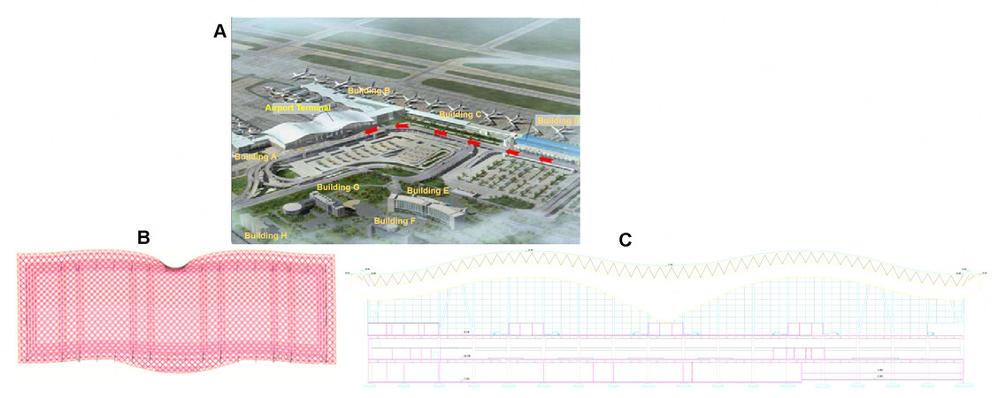
Figure 1. Terminal and adjacent buildings. (A) Google map of the terminal and its adjacent buildings; (B) plan of the terminal; (C) elevation of the terminal

Simulation of wind pressure and snow pressure coefficients

Wind-induced snow drift is a phenomenon of interactions between the near-ground wind and snow particles at the surface of ground snow and floating in the air. The classical scheme of wind-induced snow drift simulation thus includes the simulation of the near-ground wind field and the simulation of snow drift motion.

The Reynolds averaged Navier-Stokes (RANS) equations are often used to model the near-ground wind field by considering flow properties such as the wind velocity, wind pressure, flow density, wall shear stress and turbulent characteristics. To consider the effect of snow particle motion on the air turbulence characteristics and the air phase-averaged momentum, an extended two-way coupled scheme for wind-induced snow drift simulation is used. In this scheme, different damping source terms are introduced into the RANS equations and the transport equations of the turbulent kinetic energy and energy dissipation rate of the standard $$ k $$ -$$ \varepsilon $$ turbulence model ^[11]:

where $$ x $$ $$ _i $$ ($$ i $$ = 1, 2, 3) denotes the three-dimensional spatial coordinates; $$ \bar{u}_{i} $$ ($$ i $$ = 1, 2, 3) denotes the average three-dimensional components of the wind velocity; $$ \rho $$ = 1.225 kg/m$$ ^3 $$ is the flow density; $$ \bar{p} $$ is the average pressure, which depends on the design conditions of the local site; $$ v_{\mathrm{t}} $$ = 1.619 $$ \times $$ 10$$ ^{-5} $$ is the flow kinematic viscosity; $$ G_{\mathrm{k}} $$ is the production of the turbulent kinetic energy $$ k $$ , which is assumed to equal the energy dissipation rate $$ \varepsilon $$ in this study; $$ C_{1\varepsilon} $$ = 1.44 and $$ C_{2\varepsilon} $$ = 1.92 are model constants; and $$ \sigma_{\mathrm{k}} $$ = 1.0 and $$ \sigma_{\varepsilon} $$ = 1.3 are Prandtl constants relating to the turbulent kinetic energy $$ k $$ and energy dissipation rate $$ \varepsilon $$ , respectively ^[12]. $$ F_{\mathrm{i}} $$ , $$ F_{\mathrm{k}} $$ , and $$ F_{\varepsilon} $$ are respectively the damping source terms in the above three equations, which relate to the mass concentration of the snow drift, the relative velocity between moving the snow particles and air, the characteristics of snow particles and other factors ^[11]:

Here, $$ A = 3 \Phi V /\left(2 D_{\mathrm{s}} \rho_{\mathrm{s}}\right) $$ is the representative area of the obstacle related to the drag force for a mass concentration of the snow drift $$ \Phi $$ and the diameter $$ D_{\mathrm{s}} $$ = 0.5 mm and density $$ \rho_{\mathrm{s}} $$ = = 200 kg/m$$ ^3 $$ of the snow particles. $$ V $$ is the fluid volume within a unit volume; $$ C_{\mathrm{f}} $$ = 5.0 $$ \times $$ 10$$ ^3 $$ is the aerodynamic drag coefficient of the moving obstacle; $$ R_{\mathrm{p}} $$ = 0.9 is a model coefficient related to the particle speed in terms of the wind speed; and $$ C_{\mathrm{p\varepsilon}} $$ = 1.0 is a coefficient in the expression for $$ F_{\mathrm{\varepsilon}} $$ .

The simulated snowdrift is often quantified as the flux of snow erosion/deposition, which is mainly contributed by snow particles in both the saltation and suspension layers ^[13]:

The flux of snow erosion and the flux of snow deposition are expressed as ^{[14, 15]}

where $$ A_{0} $$ = 7 $$ \times $$ 10$$ ^{-4} $$ is the empirical coefficient of snow erosion/deposition; $$ u_{\mathrm{t}}^{*} $$ is the threshold friction velocity, which is considered to be lower ($$ u_{\mathrm{t}}^{*} $$ = 0.07-0.25 m/s) for fresh, loose and dry snow and during snowfall and to be higher ($$ u_{\mathrm{t}}^{*} $$ = 0.25-1.0 m/s) for older, wind-hardened, dense, and/or wet snow for which interparticle bonds and cohesion forces are strong ^[16]; $$ u^{*} $$ is the friction velocity at the snow surface, which relates to the wind velocity at a specified height obtained from the simulation of the near-ground wind field and the roughness length; and $$ w_{\mathrm{f}} $$ = 0.2 m/s is the snowfall velocity. The mass concentration of the snow drift $$ \Phi $$ is expressed by a transport equation of the snow drift based on convection-diffusion theory ^[13]:

where $$ D_{\mathrm{t}} $$ = 1.32 is the coefficient of turbulent diffusion, denoting the action of turbulent wind upon the suspended snow particles. The third term on the left side expresses convection along the height ($$ x_{k} $$ ) direction and reflects the effect of snowfall on the mass concentration of the snow drift in the suspension layer.

In representing the uneven distribution of wind and snow loads, the wind pressure and snow pressure coefficients are defined as ^{[17, 18]}

where $$ C_{\mathrm{w}} $$ ($$ x $$ , $$ t^{*} $$ ) is the wind pressure coefficient; $$ p $$ (in units of Pa) is the simulated wind pressure at point $$ x $$ on the roof; the snow-drift action time $$ t^{*} $$ is taken as 48 h herein because the lowest root-mean-square error (RMSE) of simulated points between time steps that satisfies the convergence criterion is obtained for this time step, where the RMSE values relative to the previous two time steps are both less than 0.01; $$ p_{\infty} $$ , $$ \rho_{\infty} $$ and $$ u_{\infty} $$ are respectively the wind pressure, flow density and average wind velocity at the reference position in the far field of the airshed and taken as 700.16 Pa, 1.225 kg/m$$ ^3 $$ , and 33.81 m/s (with the reference position being a 10-m height and the exponential wind profile being used as the boundary condition of the wind velocity inlet); $$ C_{\mathrm{s}} $$ ($$ x $$ , $$ t^{*} $$ ) is the snow pressure coefficient; $$ h $$ ($$ x $$ , $$ t^{*} $$ ) is the simulated snow depth at point $$ x $$ on the roof; and $$ h_{0} $$ is the ground snow depth, which is taken as 51 cm according to the average snow pressure for a 100-year return period in the design code.

The finite volume method is applied to solve the partial differential equations in Equations 1-3 and 10 using the finite element software ANSYS 14.0 FLUENT. The airshed modeling and grid division of the flow domain of the large curved roof subject to wind blowing in the most unfavorable direction (i.e., along the transverse span of the terminal building because this span is just one-third of the longitudinal span) are shown in Figure 2. The distances from the centroid of the horizontal projection plane of the terminal building to the wind inlet, outlet and top surface are set at 10 $$ L $$ , 20 $$ L $$ and 15 $$ H $$ , where $$ L $$ and $$ H $$ are the transverse dimension ($$ L $$ = 90 m) and height ($$ H $$ = 37 m) of the terminal building, respectively, and the airshed blocking rate is 1.06%. Tetrahedral elements are used to generate an unstructured mesh. A suitable grid resolution for the airshed is ensured by controlling the growth ratio of the cells from the buildings to the surrounding airshed, and the total number of cells is 1, 254, 266.

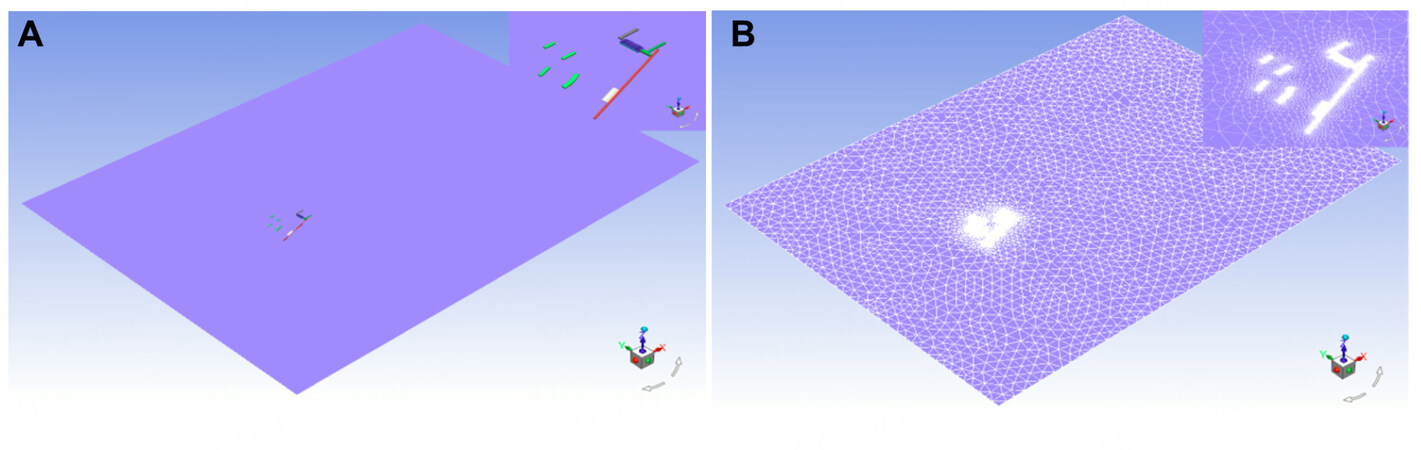
Figure 2. Modeling and mesh of the flow domain of the large curved roof subject to wind blowing in the most unfavorable direction. (A) Modeling of the flow domain; (B) mesh of the flow domain.

Figure 3 presents the coefficients of wind pressure and snow pressure on the large curved roof. For ease of analysis, the roof is divided into 18 sub-regions of the same size (36 m $$ \times $$ 30 m), which are sequentially labeled Z1 to Z18. The simulated wind pressure and snow pressure coefficients in each sub-region are the weighted values for the areas of corresponding coefficients in the region. The distribution of the wind pressure and snow pressure coefficients in sub-regions on the large curved roof is shown in Figure 4. It is seen that under the wind load of a 100-year return period, the coefficient of wind pressure on the roof is within the range [-0.77, -0.50], where the minus sign denotes a lifting force due to wind suction acting against gravity. Meanwhile, under the conditions of wind and snow loads for a 100-year return period, the snow pressure on the roof has an obvious uneven distribution. The snow pressure coefficient is within the range [0.64, 1.02], where a value exceeding 1.0 indicates snow deposition and mainly occurs in the upper-right corner of the roof near the eave. However, most of the roof area, especially the area near the ridge line in which there is much snow erosion, is subject to snow erosion.

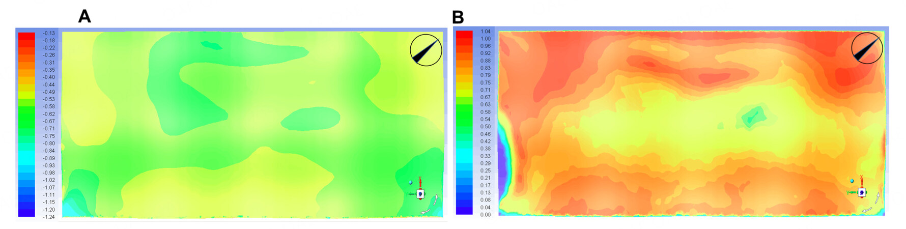
Figure 3. Coefficients of wind pressure and snow pressure on the large curved roof. (A) Wind pressure coefficient; (B) snow pressure coefficient.

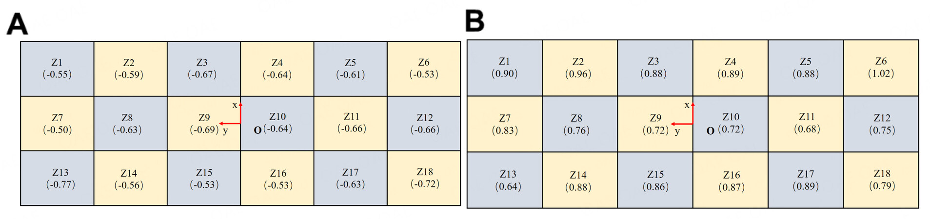
Figure 4. Distribution of coefficients of wind pressure and snow pressure in sub-regions of the large curved roof. For ease of analysis, the roof is divided into 18 sub-regions of the same size (36 m $$ \times $$ 30 m), which are sequentially labeled Z1 to Z18. (A) Wind pressure coefficient; (B) snow pressure coefficient.

The two-way coupled simulation and one-way coupled simulation were compared in the authors' previous study ^[19]. That study revealed that the two-way coupled simulation was more accurate relative to field observations (having 7.9% lower simulation error) and more efficient (having 37.1% lower computational cost) than the one-way coupled simulation.

Simulation of the fluctuating wind field

The wind pressure coefficient for the roof shown in Figure 4A is attained in steady computational fluid dynamics (CFD) simulation, and it is essentially an average value of the real wind pressure field. In reality, carrying out a transient CFD simulation is time-consuming. A practical approach is to decompose the wind field into a deterministic average wind component and a stochastic fluctuating wind component through Reynolds decomposition. The deterministic average wind component can be simulated using the RANS equations (see Equations 1-3), whereas the simulation of the stochastic fluctuating wind component often resorts to a spectral representation.

The elevation variation of the roof is far less (by two orders of magnitude) than the plan size, and the three-dimensional spatial fluctuating wind field can thus be approximately presented as a two-dimensional fluctuating wind field. Moreover, to reduce the computational cost, the same sub-regions of the roof used for the wind pressure coefficient distribution are adopted, where the center point is taken as the representative point and other points in the same sub-region are assumed to have the same fluctuating wind as the representative point. Considering the low efficiency of the conventional scheme of spectral representation methods in wind field simulation, the spectral representation method based on the wavenumber-frequency joint power spectrum and stochastic harmonic function is used in this study ^{[20, 21]}:

where $$ u $$ ($$ x $$ , $$ y $$ , $$ t $$ ) is the fluctuating wind velocity at point ($$ x $$ , $$ y $$ ) on the roof plane; $$ S^{(\mathrm{W}-\mathrm{F})} $$ is the wavenumber-frequency joint power spectrum; $$ N_{k_{x}} $$ , $$ N_{k_{y}} $$ and $$ N_\omega $$ are the numbers of discretized points in the wavenumber domains comprising $$ x $$ and $$ y $$ dimensions and the frequency domain, respectively, all of which are set at 50 in this study; ($$ k_{xi} $$ , $$ k_{yj} $$ , $$ \omega_{k} $$ ) denotes the coordinates of the $$ ijk $$ -th point in the wavenumber-frequency domain; $$ V_{ijk} $$ is the representative volume of the $$ ijk $$ -th point in the wavenumber-frequency domain; and $$ \varphi_{r, ijk} $$ ($$ r $$ = 1, 2, 3, 4) denotes mutually independent random variables uniformly distributed on [0, 2$$ \pi $$ ]. The discretized scheme of the wavenumber-frequency domain is expressed as ^[21]

where $$ \bar{k}_{xi} $$ and $$ \underline{k}_{xi} $$ are respectively the upper and lower values of the $$ i $$ -th point along the $$ x $$ dimension of the wavenumber domain; $$ \bar{k}_{yi} $$ and $$ \underline{k}_{yi} $$ are the upper and lower values of the $$ j $$ -th point along the $$ y $$ dimension of the wavenumber domain, respectively; $$ \bar{\omega}_{k} $$ and $$ \underline{\omega}_{k} $$ are respectively the upper and lower values of the $$ k $$ -th point of the frequency domain; $$ \lambda_{1} $$ , $$ \lambda_{2} $$ and $$ \lambda_{3} $$ are mutually independent random variables uniformly distributed on [0, 1]; and $$ k_{x}^{U} $$ , $$ k_{y}^{U} $$ , and $$ \omega^{U} $$ are the upper values of the wavenumber domain along the $$ x $$ and $$ y $$ dimensions and of the frequency domain, respectively, which are set at $$ \pi $$ rad/m, $$ \pi $$ rad/m and 4$$ \pi $$ rad/s. The introduction of independent random variables (i.e., $$ \lambda_{1} $$ , $$ \lambda_{2} $$ and $$ \lambda_{3} $$ ) differentiates the expression in Equation 14 from the spectral representation method based on the classical wavenumber-frequency joint power spectrum, which is referred to as the wavenumber-frequency joint power spectrum and stochastic harmonic function based spectral representation method. It is also noted from Equations 19 and 20 that an exponential formula is used in the discretized scheme of the wavenumber-frequency domain so as to retain dense point sets close to the base point and sparse point sets far from the base point.

This study uses the Davenport spectrum and coherence function model to derive the wavenumber-frequency joint power spectrum as ^[21]

where $$ U_{r} $$ is the mean wind velocity at the roof height corresponding to the 100-year return period, which is calculated as 40.35 m/s; $$ u_{*} $$ is the friction velocity, which is calculated as 2.680 m/s for the geomorphic conditions of the local site; $$ \omega $$ is the circular frequency; and $$ C_{x} $$ and $$ C_{y} $$ are the decay parameters along $$ x $$ and $$ y $$ directions, respectively, both of which are taken as 10 ^[22].

To validate the accuracy of the wavenumber-frequency joint power spectrum and stochastic harmonic function based spectral representation method, the simulated fluctuating wind velocities at three representative points on the roof, namely the center points of the sub-regions Z9 (labeled P1), Z10 (labeled P2) and Z4 (labeled P3), are considered. Representative time histories of the fluctuating wind velocities at P1, P2 and P3, and their auto-power spectra and coherence functions are shown in Figures 5 and 6. It is seen that the auto-power spectra of the simulated fluctuating wind velocities at the different spatial points and their coherence functions are in good agreement with the targets; see the Davenport spectrum and the related coherence function, which indicates that the wavenumber-frequency joint power spectrum and stochastic harmonic function based spectral representation method can be used to accurately simulate the two-dimensional fluctuating wind field for a large curved-roof structure.

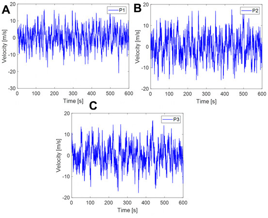
Figure 5. Representative time histories of fluctuating wind velocities at P1, P2 and P3. For ease of analysis, the roof is divided into 18 sub-regions (6 sub-regions $$ \times $$ 3 sub-regions) of the same size (36 m $$ \times $$ 30 m) that are sequentially labeled Z1 to Z18. The three representative points on the roof are P1, the center point of sub-region Z9; P2, the center point of sub-region Z10; and P3, the center point of sub-region Z4. (A) Fluctuating wind velocity at P1; (B) fluctuating wind velocity at P2; (C) fluctuating wind velocity at P3

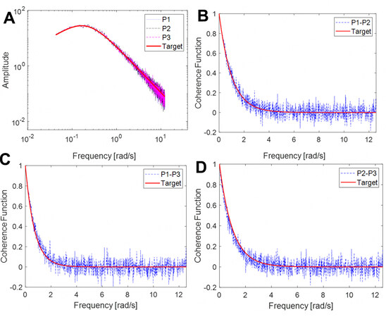
Figure 6. Auto-power spectra and coherence functions of fluctuating wind velocities at P1, P2 and P3. For ease of analysis, the roof is divided into 18 sub-regions (6 sub-regions $$ \times $$ 3 sub-regions) of the same size (36 m $$ \times $$ 30 m) that are sequentially labeled Z1 to Z18. The three representative points on the roof are P1, the center point of sub-region Z9; P2, the center point of sub-region Z10; and P3, the center point of sub-region Z4. (A) Auto-power spectra at P1, P2 and P3; (B) coherence function of P1 and P2; (C) coherence function of P1 and P3; (D) coherence function of P2 and P3

PDEM

There is randomness associated with the fluctuating wind field, and the dynamical system of the large curved-roof structure subjected to the coupled effects of the wind and snow is thus a typical random vibration problem, which needs to be solved using probabilistic methods. In this study, the PDEM, which has been widely adopted in recent years, is used to efficiently and accurately estimate the statistical information of the structural response ^[23].

Without loss of generality, we write the equation of motion of an $$ n $$ -degree-of-freedom system as

where $$ \mathbf{M} $$ is the mass matrix; $$ \mathbf{f}(\cdot) $$ is the nonlinear restoring force vector; and $$ \ddot{\mathbf{X}} $$ , $$ \dot{\mathbf{X}} $$ and $$ \mathbf{X} $$ are the acceleration, velocity and displacement of the structure relative to the ground. $$ \mathbf{F}(\cdot) $$ is the stochastic external load, where $$ \boldsymbol{\Theta} $$ is a stochastic vector representing the randomness associated with the external loads.

As regards the physical quantities $$ \mathbf{Z}=\left(\left\{Z_{j}\right\}_{j=1}^{m}\right)^{\mathrm{T}} $$ of interest (e.g., the displacement, velocity, acceleration, stress and internal force), the augmented system ($$ \mathbf{Z} $$ , $$ \boldsymbol{\Theta} $$ ) is probability preserved because all the random factors are involved. The generalized probability density evolution equation (GDEE) is thus ^[23]

Specifically, as $$ m $$ = 1, Equation 24 becomes

where $$ \boldsymbol{\theta} $$ is a sample of the stochastic vector $$ \boldsymbol{\Theta} $$ and $$ \dot{Z} $$ is the velocity of the physical quantity of interest.

It is noted that the GDEE reveals the intrinsic connections between a stochastic dynamical system and its deterministic counterpart. To solve the GDEE, an initial condition is given by

where $$ \delta $$ ($$ \times $$ ) is the Dirac delta function; $$ t_{0} $$ is the initial time; and $$ z_{0} $$ is a deterministic initial value.

Solving Equation 25 under the initial condition given as Equation 26, the instantaneous probability density function (PDF) of $$ Z(t) $$ is obtained as

where $$ \Omega_{\Theta} $$ is the sample space of the stochastic vector $$ \boldsymbol{\Theta} $$ .

The numerical procedure for solving the GDEE is as follows.

Step 1: Select the representative point set P @$$ \left\{\boldsymbol{q}_{q}=\left(q_{1, q}, q_{2, q}, \mathrm{L}, q_{\mathrm{s}, q}\right)|q=1, 2, \mathrm{L}, n_{\mathrm{pt}}\right\} $$ in the domain $$ \rm{W_{Q}} $$ , where $$ n_{\mathrm{pt}} $$ is the total number of selected points. The representative sub-domains, as a partition of $$ \rm{W_{Q}} $$ , are determined using Voronoi cells ^[24].

Step 2: For the prescribed $$ \mathbf{Q}=\boldsymbol{q}_{q} $$ , solve Equation 23 using a deterministic time integration method to evaluate $$ Z(\theta_{q}, t_{m}) $$ , where $$ t_{m} $$ = $$ m $$ D$$ t $$ , $$ m $$ = 0, 1, 2, L, and D$$ t $$ is the time step in the numerical integration.

Step 3: Introduce $$ Z(\theta_{q}, t_{m}) $$ into Equation 25 and solve the equation under the initial condition using the finite difference method with the TVD scheme to obtain the numerical solution of $$ p_{q} $$ ($$ z $$ , $$ t $$ ); i.e., $$ p_{q} $$ ($$ z_{j} $$ , $$ t_{k} $$ ), where $$ z_{j} $$ = $$ z_{0} $$ + $$ j $$ D$$ z $$ , $$ j $$ = 0, 1, 2, ..., D$$ z $$ is the space step, $$ t_{k}=k \mathrm{D} \hat{t} $$ , $$ k $$ = 0, 1, 2, ... and $$ \mathrm{D} \hat{t} $$ is the time step in the finite difference method.

Step 4: Obtain the numerical result of $$ p_{z} $$ ($$ z $$ , $$ t $$ ) using Equation (27); i.e.,

Finite element modeling and analysis

Using the finite element analysis platform SAP2000 v19, the deterministic structural dynamic analysis involved in Step 2 in Section 3.1 is carried out. In the concrete frame-steel roof hybrid structure, the lower concrete structure has higher rigidity than the top large-span steel roof structure, and the structural internal force and displacement are generally small under wind and snow loads. To simplify the calculation, therefore, only the steel roof at the top of the terminal building is modeled using finite elements, and the bottom of the steel pipe column and steel diagonal bracing adopts hinge supports, of which the number is 58. For the steel pipe columns, steel diagonal bracings, upper chords, lower chords and diagonal rods of the steel roof, frame elements are used, and the section size of each element is selected according to the actual design size. The steel roof support shell adopts massless shell elements for roof load transfer. By doing so, the finite element model of the large curved-roof structure includes a total of 4241 nodes, 16, 073 frame elements and 3083 massless shell elements, with a total structural mass of 2924.6 t. The three-dimensional finite element model is shown in Figure 7A.

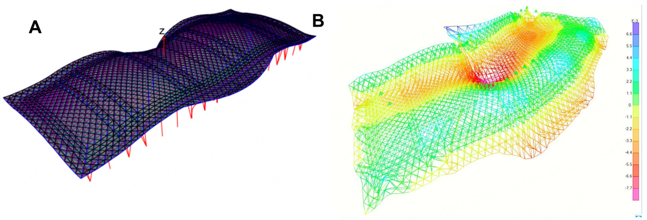
Figure 7. Three-dimensional finite element model and the first mode of the structure. (A) View of the finite element model; (B) first mode of the structure.

To clarify the basic dynamic characteristics of the large curved-roof structure, structural modal analysis is carried out using the Rayleigh-Ritz vector method. It is found that the first four orders of the modal frequencies are 0.854, 0.767, 0.553 and 0.463 s, and they sequentially correspond to the modal characteristics of horizontal vibration along the $$ y $$ axis, horizontal vibration along the $$ x $$ axis and torsional and vertical vibrations along the $$ z $$ axis. The first mode is shown in Figure 7B. It is seen that the basic natural vibration period of the structure is higher than 0.25 s for the basic natural vibration period of flexible structures according to Chinese Technical Regulation for Spatial Grid Structures (JGJ7-2010); therefore, the wind-induced vibration problem should be considered in the structural analysis. Additionally, the natural vibration periods of the structure are distributed in a narrow range; i.e., the structure has densely distributed frequencies. Thereby, the contribution of each mode to the dynamic response of the structure is equally important, and ignoring the contribution of high-order modes will inevitably lead to large computational errors. Moreover, the overall vertical stiffness of the structure is high, and it is predicted that the vertical deflection of nodes of the roof under the loads will be smaller than that for a flexible roof of the same size.

As a practical situation, the large curved-roof structure is simultaneously subjected to the wind load comprising average and fluctuating wind components, the snow load unevenly distributed on the roof and the self-weight load. Structural analysis should consider a certain combination of the effects of these loads. In this study, they are in weighted linear combination according to Chinese Load Code for the Design of Building Structures (GB50009-2012). Figure 8A and B show the steady member axial stress and node vertical deflection of the large curved-roof structure under representative wind, snow and self-weight loads (at a time instant of 300 s).

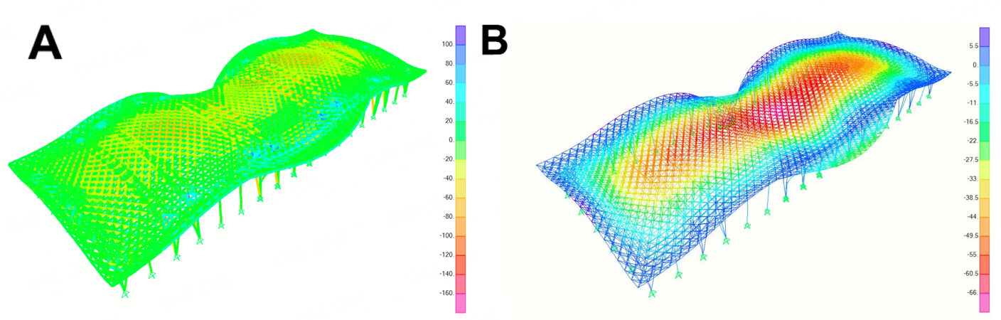
Figure 8. Steady member axial stress and node deflection of the large curved-roof structure under representative wind, snow and self-weight loads (at a time instant of 300 s). (A) Member axial stress of the structure (MPa); (B) node vertical deflection of the structure (mm).

It is seen that under the representative wind, snow and self-weight loads, the axial stress acting on members is in the range of -198 to 154 MPa, and the lower roof chord and roof inclined rod experience higher stresses as same as the range in the structural level, whereas the upper roof chord and roof support column experience lower stresses in the range of -141 to 106 MPa. Under the representative wind, snow and self-weight loads, the node vertical deflection is in the range of -71.5 to 16.5 mm and the deflection is a maximum at the nodes in the mid-span area of the roof, whereas the overhanging part of the roof has a small upward deflection. Therefore, the member axial stress of the large curved-roof structure reaches a maximum of 198 MPa, and the node vertical deflection reaches a maximum of 71.5 mm. Considering that the strength of the structural member is 345 MPa, the maximum member axial stress is approximately 0.574 times the maximum allowable stress. The threshold of the node vertical deflection is 1/250 of the horizontal span of the structure according to the design provision (i.e., 300 mm), and the maximum node vertical deflection is approximately 0.238 times the threshold. The member axial stress is closer to its limit value than the node vertical deflection, and the risk of the member yielding is thus higher than that of node deflection, which is in agreement with the results of structural modal analysis.

Statistical analysis of the stochastic responses of structures

In this study, there is a random vibration problem due to the randomness associated with the fluctuating wind field. Using the PDEM, a total of 300 samples of the fluctuating wind field are simulated and used for the stochastic response analysis and reliability assessment of the large curved-roof structure. For the purpose of illustration, the stochastic responses of sub-region Z10 are addressed. Time histories of the means and standard deviations of the axial stress of Member #14294 and the vertical deflection of Node #3019 in this sub-region are presented in Figure 9A-D, respectively. The simulated fluctuating wind field is a stationary state, and the time histories of statistical moments within just the first 300 s are thus presented to clearly show the initial non-stationary stage of the structural responses.

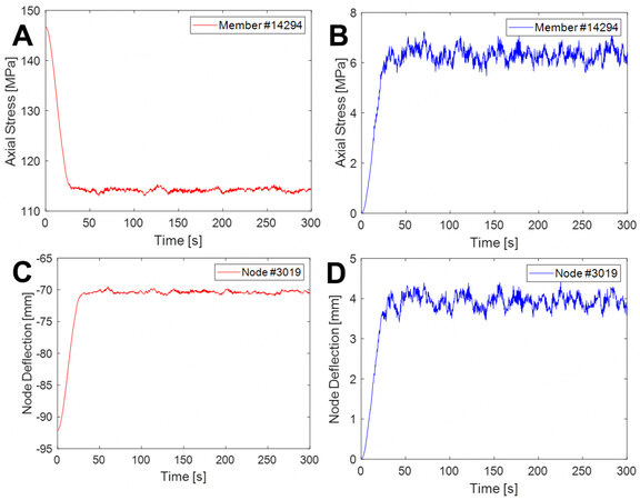
Figure 9. Time histories of the means and standard deviations of the axial stress acting on Member #14294 and vertical deflection of Node #3019 in sub-region Z10. For ease of analysis, the roof is divided into 18 sub-regions (6 sub-regions $$ \times $$ 3 sub-regions) of the same size (36 m $$ \times $$ 30 m) that are sequentially labeled Z1 to Z18. (A) Mean of the axial stress acting on a member stress acting on a member; (B) standard deviation of the axial; (C) mean of the vertical deflection of a node; (D) Standard deviation of the vertical deflection of a node.

It is seen that the means and standard deviations of the member axial stress and node vertical deflection quickly reach a steady state; i.e., within 50 periods of the basic natural vibration of the structure. Additionally, the average wind component of the stochastic wind load has a suction effect on the roof, which partially offsets the structural response relating to the self-weight load and the unevenly distributed snow load, and the average wind component thus reduces the overall response of the structure. Meanwhile, the fluctuating wind component has an appreciable dynamic effect on the responses of the structure. Furthermore, the probability densities of the axial stress of Member #14294 at 100, 200, and 300 s and in the time interval [150, 160] s are presented in Figure 10. It is seen that the probability density of the structural response in the stage of the steady state only slightly changes and approximately follows a normal distribution. This can be explained in that the simulation of the stochastic wind field is a Gaussian process and the dynamic analysis using finite element software reveals the linear state of the structure.

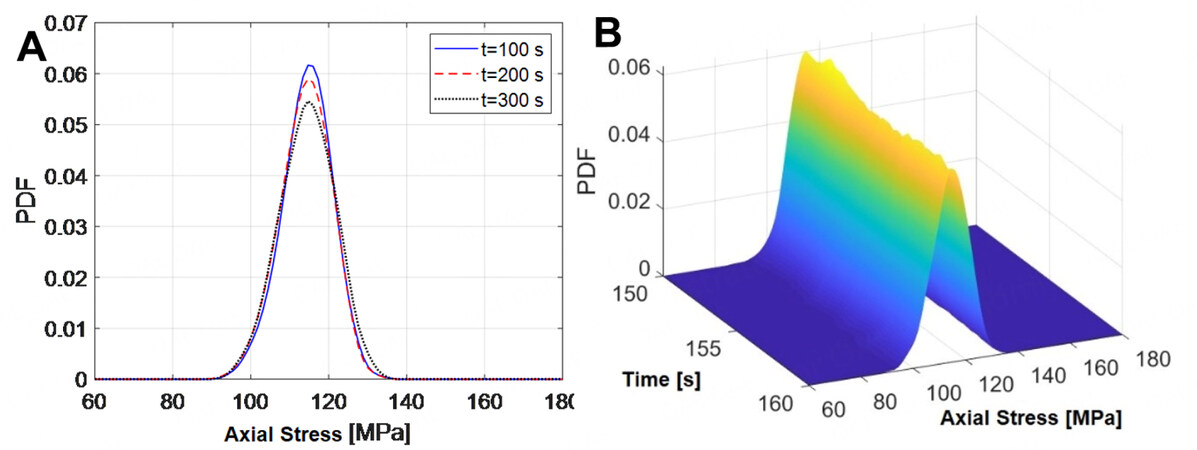
Figure 10. Probability densities of the axial stress of Member #14294. (A) Probability densities at typical instants; (B) probability densities in the time interval [150, 160] s.

Figure 10 also shows that although the mean of the member axial stress is far less than the maximum allowable stress, the member still faces the possibility of yielding because the axial stress varies appreciably. It is thus necessary to carry out reliability assessment in terms of the member axial stress in determining the safety of the structure.

PDEM-based reliability method

Without loss of generality, the associated reliability of the first-passage problem of structural dynamical systems is defined as

where Pr$$ \{\times \}$$ is the probability operator of a random event; $$ Z $$ ($$ \boldsymbol{\Theta} $$ , $$ t $$ ) is the random event of physical quantities of concern such as the stress, internal force and deflection; $$ \Omega_{s} $$ is the safe domain; and $$ T $$ is the time duration corresponding to $$ Z $$ ($$ \cdot $$ ).

When the structural system has multiple modalities of failure, the first-passage problem is expressed as

where $$ m $$ is the number of random events and $$ \left\{Z_{B i}\right\}_{i=1}^{m} $$ denotes the safe thresholds of the random events $$ \left\{Z_{i}(\boldsymbol{\Theta}, t)\right\}_{i=1}^{m} $$ . For the convenience of description, we refer to the single-passage level as a type-B barrier herein.

We construct an equivalent extreme-value event as a random variable:

The reliability function in Equation 29 can then be defined alternatively as

Equation (32) can be rewritten as

where $$ p_{Z_{\mathrm{eq}}}(z, T) $$ is the PDF of $$ Z_{\mathrm{eq}}(\boldsymbol{\Theta}, T) $$ .

Therefore, the introduction of the equivalent extreme-value event criterion (see Equation 31) reduces the high-dimension integral associated with the reliability of systems into the one-dimension integral ^[25].

To derive the PDF of the equivalent extreme-value event, a pseudo-random process is first defined as

which satisfies the conditions

where $$ \tau $$ denotes the generalized time and $$ \tau_{0} $$ , $$ \tau_{c} $$ denote the initial and final time instants of the pseudo-random process, respectively.

Theoretically, arbitrary forms of the pseudo-random process $$ Y(\tau) $$ can be assumed if they satisfy the conditions shown in Equation 35. This study uses the form $$ Y(\tau) $$ = $$ Z_{\mathrm{eq}}(\boldsymbol{\Theta} $$ , $$ t $$ )sin($$ \omega\tau $$ ), where $$ \omega $$ = 2.5$$ \pi $$ , $$ \tau_{c} $$ = 1.

It is observed that the probabilistic information of the equivalent extreme-value event $$ Z_{\mathrm{eq}}(\boldsymbol{\Theta}, T) $$ is completely included in the final time instant of the pseudo-random process $$ Y(\tau) $$ , and they share the same randomness denoted by $$ \boldsymbol{\Theta} $$ . Therefore, the augmented system ($$ Y(\tau) $$ , $$ \boldsymbol{\Theta} $$ ) is a probability conservation system that is governed by the equation for the generalized probability density evolution given as Equation 25; thereby, the PDF of the pseudo-random process (i.e., $$ p_{Y} $$ ($$ y $$ , $$ \tau $$ )) can be derived. One then has

Reliability assessment of a structure

Using the PDEM and the associated reliability method, the PDFs and cumulative density functions (CDFs) of the equivalent extreme-value axial stress of members in the sub-regions Z1, Z8, Z10 and Z17 are derived, as shown in Figure 11. It is seen that all the curves related to the sub-regions under investigation are far below the maximum allowable stress (i.e., 345 MPa), indicating safety in these regions. It is also seen that among the four representative sub-regions under investigation, the sub-region Z10 has the largest member axial stress, followed by Z1, Z8 and Z17 in order. In view of Figure 4, the sub-region Z1 features lower wind suction and higher snow pressure and is thus expected to have appreciable member axial stress, whereas the other three sub-regions feature almost similar wind suction and snow pressure and thus, compared with Z8 and Z17, the sub-region Z10 has a greater contribution from the fluctuating wind component to the member axial stress because this area is located in the rolling region of the curved roof. Furthermore, all the sub-regions are analyzed and their reliabilities are shown in Figure 12. Additionally, the PDF and CDF of the equivalent extreme-value axial stress of members of the roof structure are presented in Figure 13, Showing a safe structure in the global sense.

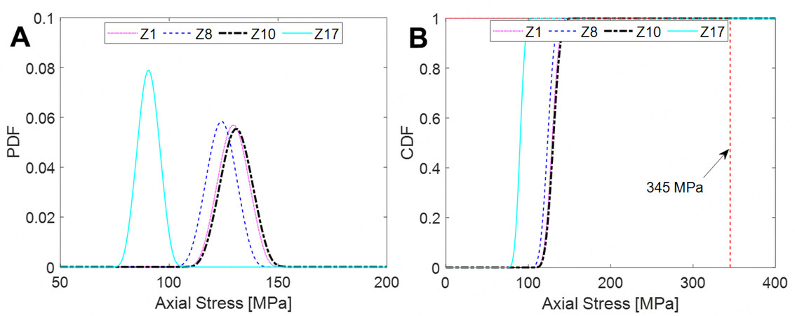
Figure 11. PDFs and CDFs of the axial stress acting on members in sub-regions Z1, Z8, Z10 and Z17. For ease of analysis, the roof is divided into 18 sub-regions (6 sub-regions $$ \times $$ 3 sub-regions) of the same size (36 m $$ \times $$ 30 m) that are sequentially labeled Z1 to Z18; PDF: probability density function; CDF: cumulative density function. (A) PDFs of the equivalent extreme-value axial stress; (B) CDFs of the equivalent extreme-value axial stress.

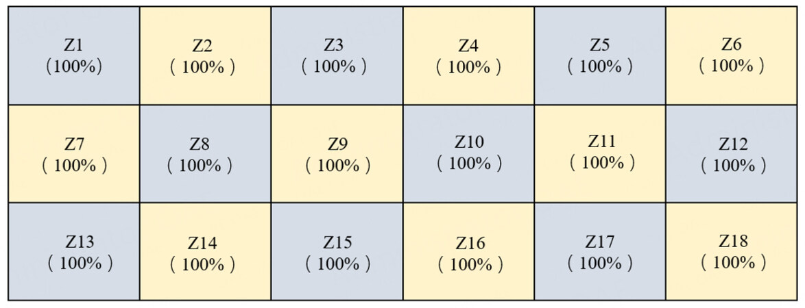
Figure 12. Reliabilities of axial stress of members in sub-regions of the roof structure. For ease of analysis, the roof is divided into 18 sub-regions of the same size (36 m $$ \times $$ 30 m) that are sequentially labeled Z1 to Z18.

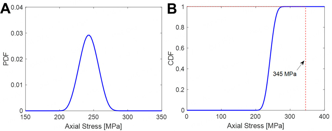
Figure 13. PDF and CDF of equivalent extreme-value axial stress of members of the roof structure. (A) PDF of equivalent extreme-value axial stress; (B) CDF of equivalent extreme-value axial stress. PDF: Probability density function; CDF: cumulative density function.

In summary, under stochastic wind, snow and self-weight loads with a 100-year return period, the equivalent extreme-value axial stresses of members in each sub-region and in the global structural system are both far less than the maximum allowable stress, and the large curved roof structure is deemed to be sufficiently safe.

Acknowledgments

The support of the National Key R & D Program of China (Grant No. 2017YFC0803300) is highly appreciated.

Authors' contributions

Conceptualization, methodology, validation, formal analysis, writing - review & editing, resources, supervision, project administration: Peng Y

Software, investigation, data curation: Zhao W, Zhou J

Methodology, writing - original draft, visualization: Zhao W

Availability of data and materials

Some or all data and materials that support the findings of this study are available from the corresponding author upon reasonable request.

Financial support and sponsorship

National Key R & D Program of China (Grant No. 2017YFC0803300).

Conflicts of interest

All authors declared that there are no conflicts of interest.

Ethical approval and consent to participate

Not applicable.

Consent for publication

Not applicable.

Copyright

© The Author(s) 2022.

REFERENCES

1. Vazna RV, Zarrin M. Sensitivity analysis of double layer Diamatic dome space structure collapse behavior. Eng Struct 2020;212:110511.
2. Wang XJ, Li QS, Yan BW, Li JC. Field measurements of wind effects on a low-rise building with roof overhang during typhoons. J Wind Eng Ind Aerodyn 2018;176:143-57.
3. Zhou XY, Li XF. Simulation of snow drifting on roof surface of terminal building of an airport. Available from: https://www.researchgate.net/publication/285439767_Simulation_of_Snow_Drifting_on_Roof_Surface_of_Terminal_Building_of_an_Airport . [Last accessed on 5 Dec 2022].
4. Zhang GL, Zhang QW, Fan F, Shen SZ. Numerical simulations of snowdrift characteristics on multi-span arch roofs. J Wind Eng Ind Aerodyn 2021;212:104593.
5. Aghamohammadi R, Nasrollahzadeh K, Mofidi A, Gosling P. Reliability-based assessment of bond strength models for near-surface mounted FRP bars and strips to concrete. Compos Struct 2021;272:114132.
6. Zhang GL, Zhang QW, Fan F, Shen SZ. Numerical simulations of development of snowdrifts on long-span spherical roofs. Cold Reg Sci Technol 2021;182:103211.
7. Zhang GL, Zhang QW, Fan F, Shen SZ. Field measurements of snowdrift characteristics on reduced scale building roofs based on the size effect study. Structures 2021;32:2020-31.
8. Liu DT, Wang B, Li YL, Liu S. A source term model for drifting snow based on the assumption of local equilibrium saltation. Cold Reg Sci Technol 2021;181:103175.
9. Yang QS, Chen B, Wu Y, Tamura Y. Wind-induced response and equivalent static wind load of large-size curved-roof structures by combined Ritz-proper orthogonal decomposition method. J Struct Eng 2013;139:997-1008.
10. Uematsu Y, Watanabe K, Sasaki A, Yamada M, Hongo T. Wind-induced dynamic response and resultant load estimation of a circular flat roof. J Wind Eng Ind Aerodyn 1999;83:251-61.
11. Okaze T, Takano Y, Mochida A, et al. Development of a new k-epsilon model to reproduce the aerodynamic effects of snow particles on a flow field. J Wind Eng Ind Aerodyn 2015;144:118-24.
12. Alfonsi G. Reynolds-Averaged Navier-Stokes equations for turbulence modeling. Appl Mechan Rev 2009;62:040802.
13. Uematsu T, Nakata T, Takeuchi K, et al. Three-dimensional numerical simulation of snowdrift. Cold Reg Sci Technol 1991;20:65-73.
14. Anderson RS, Haff PK. Wind modification and bed response during saltation of sand in air. Acta Mechan 1991:21-51.
15. Naaim M, Naaim-Bouvet F, Martinez H. Numerical simulation of drifting snow: erosion and deposition models. Ann Glaciol 1998;26:191-6.
16. Kind RJ. Snow drifting. In Gray DM, Male DH, editors. Handbook of Snow, principles, processes, management, and use. Oxford: Pergamon Press; 1981, pp. 338-59.
17. Zhou XY, Zhang Y, Kang L, et al. CFD simulation of snow redistribution on gable roofs: impact of roof slope. J Wind Eng Ind Aerodyn 2019;185:16-32.
18. Sun X, He R, Wu Y. Numerical simulation of snowdrift on a membrane roof and the mechanical performance under snow loads. Cold Reg Sci Technol 2018;150:15-24.
19. Peng YB, Zhao WJ, Li S, Zhou J. Prediction of wind-induced snow redistribution on large-span building roof based on two-way coupled simulation. Nat Hazards Rev 2022. under review.
20. Song YP, Chen JB, Peng YB Spanos PD, Li J. Simulation of nonhomogeneous fluctuating wind speed field in two-spatial dimensions via an evolutionary wavenumber-frequency joint power spectrum. J Wind Eng Ind Aerodyn 2018;179:250-9.
21. Chen JB, Song YP, Peng YB, et al. Simulation of homogeneous fluctuating wind field in two spatial dimensions via a joint wave number-frequency power spectrum. J Eng Mechan 2018;144:04018100.
22. Peng YB, Wang SF, Li J. Field measurement and investigation of spatial coherence for near-surface strong winds in Southeast China. J Wind Eng Ind Aerodyn 2018;172:423-40.
23. Li J, Chen JB. Stochastic dynamics of structures. Singapore: John Wiley & Sons; 2009.
24. Chen JB, Ghanem R, Li J. Partition of the probability space in probability density evolution analysis of non-linear stochastic structures. Probabilistic Eng Mech 2009;24:27-42.
Cite This Article
Export citation file: BibTeX | RIS
OAE Style
Peng Y, Zhao W, Zhou J. Reliability analysis of a large curved-roof structure considering wind and snow coupled effects. Dis Prev Res 2022;1:8. http://dx.doi.org/10.20517/dpr.2022.02
AMA Style
Peng Y, Zhao W, Zhou J. Reliability analysis of a large curved-roof structure considering wind and snow coupled effects. Disaster Prevention and Resilience. 2022; 1(2): 8. http://dx.doi.org/10.20517/dpr.2022.02
Chicago/Turabian Style
Peng, Yongbo, Weijie Zhao, Jian Zhou. 2022. "Reliability analysis of a large curved-roof structure considering wind and snow coupled effects" Disaster Prevention and Resilience. 1, no.2: 8. http://dx.doi.org/10.20517/dpr.2022.02
ACS Style
Peng, Y.; Zhao W.; Zhou J. Reliability analysis of a large curved-roof structure considering wind and snow coupled effects. Dis. Prev. Res. 2022, 1, 8. http://dx.doi.org/10.20517/dpr.2022.02
About This Article
Special Issue
Copyright
Data & Comments
Data
Cite This Article 14 clicks
Like This Article 10
likes
Comments
Comments must be written in English. Spam, offensive content, impersonation, and private information will not be permitted. If any comment is reported and identified as inappropriate content by OAE staff, the comment will be removed without notice. If you have any queries or need any help, please contact us at support@oaepublish.com.